American Economic Review 2016, 106(10): 2982–3028
http://dx.doi.org/10.1257/aer.20151052
2982
* Hurst: Booth School of Business, University of Chicago, 5807 S. Woodlawn Ave., Chicago, IL 60637 (e-mail:
Chicago, IL 60637 (e-mail: [email protected]); Seru: Booth School of Business, University of Chicago, 5807
University of Chicago, 5807 S. Woodlawn Ave., Chicago, IL 60637 (e-mail: joseph.va[email protected]). We
thank Sumit Agarwal, Heitor Almeida, Tom Davidoff, John Driscoll, Matthew Kahn, Arvind Krishnamurthy, John
Leahy, Tomasz Piskorski, Stijn Van Nieuwerburgh, Monika Piazzesi, David Scharfstein, Johannes Stroebel, Adi
Sunderam, Francesco Trebbi, and seminar participants at Berkeley Haas, Einaudi Institute, Federal Reserve Board,
HEC, Indian School of Business, Kellogg, MIT, National University of Singapore, NBER Monetary Economics
Program Meeting, Ohio State, NBER Summer Institute, Chicago Fed, Rutgers, Stanford, Toronto, UBC, UCLA,
University of Chicago Booth, University of Chicago Harris, University of Illinois, University of Michigan, Wharton,
the FRIC 2014 conference on nancial frictions, and the NBER conference on Financing Housing Capital for help-
ful comments and suggestions.
†
Go to http://dx.doi.org/10.1257/aer.20151052 to visit the article page for additional materials and author
disclosure statement(s).
Regional Redistribution through
the US Mortgage Market
†
By E H, B J. K, A S, J V*
Regional shocks are an important feature of the US economy.
Households’ ability to self-insure against these shocks depends on
how they affect local interest rates. In the United States, most bor-
rowing occurs through the mortgage market and is inuenced by the
presence of government-sponsored enterprises (GSE). We establish
that despite large regional variation in predictable default risk, GSE
mortgage rates for otherwise identical loans do not vary spatially.
In contrast, the private market does set interest rates which vary
with local risk. We use a spatial model of collateralized borrowing to
show that the national interest rate policy substantially affects wel-
fare by redistributing resources across regions. (JEL E32, E43, G21,
G28, L32, R11, R31)
The Great Recession has led to wide disparities in economic activity across regions
within the United States. The extent to which households can borrow to self-insure
against these regional shocks depends crucially on the interest rate and how it var-
ies with regional economic conditions. Theoretical models typically assume that
regions within a monetary union share a common risk-adjusted interest rate.
1
Yet,
there are no papers—of which we are aware—testing whether risk-adjusted interest
rates are equated across regions within a monetary union like the United States.
In this paper, we use data on mortgage loans, which represent the bulk of household
borrowing, to document two new facts. First, risk-adjusted rates are not equalized
1
The theoretical literature that assumes a constant risk-adjusted (or risk-free) interest rate across regions is
extensive. Recent papers making this assumption in the macroeconomics, monetary union, and public nance liter-
atures include: Lustig and Van Nieuwerburgh (2005); Farhi and Werning (2014); Nakamura and Steinsson (2014);
Yagan (2016); Zidar (2015); and Beraja, Hurst, and Ospina (2016).
2983
Hurst et al.: regional redistribution
Vol. 106 no. 10
across locations within the US monetary union: despite large regional variation in
ex ante predictable default risk, there is no regional variation in mortgage contract
rates for loans securitized by government-sponsored enterprises (GSE). Since GSEs
securitize most of the loans in the US mortgage market, this constant contract rate
in the face of variation in predictable default risk implies that the majority of bor-
rowers face risk-adjusted rates which do vary with their locations. Second, this lack
of risk-based pricing does not occur because this risk cannot be observed ex ante: we
show that otherwise similar non-GSE loans that are securitized in the private market
increase (decrease) mortgage rates when ex ante local default risk rises (falls).
If mortgage rates do not respond to local economic shocks that increase ex ante
default risk, then individuals in those regions face lower borrowing costs than they
otherwise would if default risk was priced into interest rates. This reduction in bor-
rowing costs may in turn offset some of the negative local economic shock that
increased default risk in the rst place. Conversely, individuals in regions with
low default risk will face higher borrowing costs than if this low default risk was
priced into interest rates. Thus, the constant interest rate policy followed by the
GSEs results in state-contingent regional transfers. While the rst half of our paper
concentrates on documenting the constant interest rate policy, the second half of the
paper quanties the size and welfare consequences of these implicit transfers.
Our paper unfolds in three parts. We begin by using detailed loan-level data secu-
ritized by the GSEs to show that local characteristics systematically predict future
local loan default even after controlling for other observable borrower and loan
characteristics. For example, there is medium-run persistence in local default prob-
abilities: conditional on borrower and loan characteristics, regions that experienced
higher default rates yesterday are more likely to experience higher default rates
tomorrow. These ndings hold throughout the entire 2000s and are not limited to the
period surrounding the 2008 recession. Despite this nding, we further document
that interest rates on loans securitized by the GSEs do not vary at all with this pre-
dictable default risk. These patterns hold across different time periods and are robust
to many different specications to predict local mortgage default rates. The results
are striking. Even though the GSEs charge different interest rates to borrowers who
take on greater leverage (i.e., have higher loan-to-value (LTV) ratios) or who are
less credit-worthy (i.e., have lower FICO scores), they do not charge higher rates
to borrowers in regions with declining economic conditions even though they are
much more likely to eventually default. Additionally, we show that local mortgage
rates for loans securitized by the GSEs do not vary with other dimensions that could
also induce local adjustment for risk, such as local mortgage recourse laws, local
bankruptcy laws, or local lender concentration.
In the second part of the paper, we then provide an assessment of the extent to
which GSE interest rates should vary spatially, given the large spatial variation in
default risk. To do this, we exploit loan-level data containing loans securitized by pri-
vate agencies. To facilitate comparisons, we focus on a set of loans which we refer to
as “prime jumbo” loans. The GSEs are only allowed to securitize loans smaller than
some threshold size, known as the conforming loan limit. Our prime jumbo loans
are larger than those made by the GSEs but comparable on many other dimensions
(in particular, FICO score and LTV ratio). Unlike the interest rate on GSE loans, we
document that the interest rate on prime jumbo loans rises dramatically with ex ante
2984
THE AMERICAN ECONOMIC REVIEW
OCTObER 2016
local predicted default risk. Thus, although there is no regional risk-based pricing in
the government-backed GSE market, the private market does set interest rates based
in part on regional risk factors. This result shows that local risk factors are ex ante
observable by lenders.
Employing a variety of techniques, including a regression discontinuity approach
around the conforming limit threshold, we construct counterfactual estimates of the
extent to which GSE mortgage rates should have varied across regions within the
United States. In particular, we construct these estimates during both the early 2000s
and during the Great Recession, assuming that the GSEs priced local risk similarly
to the private market. These results are robust to controlling for many potential con-
founding factors, including the possibility that prepayment propensities or points
and fees vary spatially. We also document that loan amounts for GSE and prime
jumbo borrowers do not respond differentially to ex ante predictable default. This
suggests that, relative to the private market, the GSE market does not compensate
for the lack of spatial variation in mortgage rates by reducing the amount of credit
extended.
We explore a number of explanations for why the relationship between mortgage
rates and predictable default differs in the GSE and private markets. We conclude
that political pressure is the most reasonable explanation for the patterns we observe.
The GSEs face a great deal of political scrutiny: we provide evidence showing that
multiple times during the past decade the GSEs tried to implement space-based
policies but that these efforts were abandoned after backlash from Congress, real-
tors, and community groups that objected to GSEs using different standards across
regions.
2
The fact that risk-adjusted mortgage rates are not equalized across regions implies
that resources are redistributed across regions through the mortgage market. In the
nal part of the paper, we quantify the economic impact of the transfers induced by
the GSEs’ constant interest rate policy. We begin with a simple back-of-the-envelope
exercise that “ marks-to-market” the interest rate on GSE-securitized loans origi-
nated during the Great Recession. More precisely, for each loan, we calculate the
difference between the actual mortgage payment we observe under the GSE constant
interest rate policy and the counterfactual mortgage payment if GSE interest rates
instead priced local predicted default like the private market. Summing up these
wedges over all loans originated during the Great Recession implies a total redistri-
bution of $14.5 billion in mortgage payments across regions during the 2007–2009
period. While this calculation already suggests an important redistributive role for
the constant interest rate policy, it does not fully account for the total effects of the
policy. In particular, it ignores: (i) equilibrium effects of the GSE policy on local
income and house prices; (ii) equilibrium effects associated with households adjust-
ing their housing and mortgage behavior in response to changes in the GSE pricing
rule; and (iii) the effect of the policy on loans originated outside of the 2007–2009
period.
2
This lack of local variation in pricing rules appears in many pricing decisions for the US government. For
example, the US Postal Service charges the same at rate for all rst-class mail regardless of the distance traveled.
Finkelstein and Poterba (2014) also nd that political economy considerations can explain why UK insurance pro-
viders price nationally despite the presence of local drivers of mortality risk.
2985
Hurst et al.: regional redistribution
Vol. 106 no. 10
In order to provide a more complete account of the welfare consequences of the
constant interest rate policy, we build a structural model suitable for counterfactual
analysis. This spatial model of collateralized borrowing has households that face
region-specic shocks to house prices and labor earnings as well as purely idiosyn-
cratic labor earnings risk. Individuals in the model can choose whether to own a
home or to rent, in addition to choosing nondurable consumption and liquid savings
over their life cycle. Owner-occupied housing is subject to xed adjustment costs
but serves as collateral against which individuals can borrow to smooth nondurable
consumption. In addition, changes in interest rates have effects on local house prices
and income.
We use this model to assess the welfare consequences of the GSEs’ constant
interest rate policy. In particular, we ask what would happen if the GSEs maintained
their role in the mortgage market but simply allowed interest rates to vary with local
default risk as in the private market.
3
Within the model, we compare two scenarios,
one in which a common interest rate applies to all regions and one in which interest
rates respond to the local default risk within each region. We use the empirical work
in the rst part of the paper to discipline the counterfactual interest rate policy in
which rates respond to local default risk.
In our benchmark calibration, designed to match the regional variation observed
during the Great Recession, the GSEs’ pricing policy generates a present value
effect roughly equivalent to a one-time $1,000 per-household tax on a region with a
two-standard-deviation increase in regional activity (i.e., decline in predicted local
mortgage default) and generates a one-time subsidy of $900 for a region with a
two-standard-deviation decrease in regional activity (i.e., increase in predicted local
mortgage default). This one-time net transfer of $1,900 per household from regions
with two-standard-deviation positive shocks to those with two-standard-deviation
negative shocks is larger than the per-household tax rebate checks paid by the US
government during the 2001 and 2008 recessions. Thus, our results suggest that
the magnitude of redistribution induced by the GSEs through the mortgage mar-
ket is economically meaningful and compares in size to transfer policies that have
received vastly more attention.
Rather than focusing on the model’s implications for particular regions during
the Great Recession, we can also add up the total transfers across all regions. Under
our baseline calibration, our model implies that about $47 billion is transferred via
the mortgage market from regions receiving better than average economic shocks to
regions receiving worse than average economic shocks. The model-implied transfers
are higher than our estimated back-of-the-envelope transfers, in large part because
the model allows for the constant interest rate policy to provide an additional benet
to local economic activity by boosting local income and house prices.
We also show that this large average transfer across regions hides substantial
heterogeneity in the effects within regions since not all households have equal mort-
gage exposure. In particular, our model implies that the GSE pricing policy has a
much larger effect on middle-aged households than on young households because
3
To be clear, we are not evaluating the consequences of eliminating GSEs and are instead considering a simple
change in their interest rate policy. Eliminating GSEs would have many important effects on housing markets, as
described in Elenev, Landvoigt, and Van Nieuwerburgh (2016).
2986
THE AMERICAN ECONOMIC REVIEW
OCTObER 2016
the young mostly choose to rent and are thus less sensitive to the local mortgage
rate. Similarly, the implied transfer is largest for middle-income households within
each region, as the poorest households do not own houses and the richest households
have little mortgage debt. Thus, the GSE constant interest rate policy has the great-
est effects on the middle class.
Our work relates to a number of existing literatures. First, there is a small body of
work that studies the extent to which risk is shared across US states through credit
markets. For example, Asdrubali, Sorensen, and Yosha (1996) examine risk sharing
across US states and suggest that credit markets smooth about 23 percent of regional
shocks. In that paper, the key mechanism is general borrowing and lending across
regions. Lustig and Van Nieuwerburgh (2010) directly explore the role of housing
equity in supporting regional risk sharing. As housing equity increases, households
are better able to borrow. The increased ability to borrow relaxes local liquidity
constraints, allowing local residents to better insure themselves against local shocks.
Lustig and Van Nieuwerburgh nd that the extent of regional risk sharing varies with
the state of the aggregate housing market. Our paper complements these ndings by
highlighting a direct mechanism by which the credit market serves to insure regional
shocks. This mechanism, as far as we can tell, is a novel addition to the regional
risk-sharing literature.
4
Additionally, our paper speaks to how local shocks are mitigated within monetary
and scal unions. This question has gained considerable attention in recent years as
large disparities in regional outcomes have occurred within both the United States
and Europe. There is a large literature arguing that an integrated tax and transfer
system together with easy factor mobility can help mitigate local shocks.
5
Most
papers exploring regional variation in economic conditions impose constant interest
rates across regions. Since these models typically do not include default risk, this
should be interpreted as imposing a common risk-adjusted rate. Our work suggests
that institutional features—such as the political pressure faced by GSEs—may lead
to violations of this assumption. The bulk of US household borrowing occurs in
mortgages securitized by GSEs. We show that loans securitized by the GSEs exhibit
contract rate equalization across regions, but that default risk varies substantially
across these same regions. This implies that the risk-adjusted rate on these loans
varies substantially. This in turn leads to quantitatively important transfers across
regions that occur in state-contingent ways.
4
More broadly, our work contributes to the growing literature emphasizing that housing nance has import-
ant implications for the US economy. Recent papers in this literature include Agarwal et al. (2012); Di Maggio,
Kermani, and Ramcharan (2015); Keys et al. (2014); Lustig and Van Nieuwerburgh (2005); Mian, Su, and Trebbi
(2015); Mian, Rao, and Su (2013); Mayer, Pence, and Sherlund (2009); Piazzesi, Schneider, and Tuzel (2007);
and Scharfstein and Sunderam (2013).
5
See, for example, Farhi and Werning (2012) and the citations within. Additionally, Sala-i-Martin and Sachs
(1991) and Asdrubali, Sorenson, and Yosha (1996) explore the role of an integrated scal system in smoothing
income across US states. For a classic example of the importance of factor mobility, see Blanchard and Katz (1992).
Recent examples include Farhi and Werning (2014); Charles, Hurst, and Notowidigdo (2016); and Yagan (2016).
Also see Feyrer and Sacerdote (2011) for arguments that the integrated tax and transfer system as well as the ease
of factor mobility are reasons for the long-run stability of the monetary union across US states.
2987
Hurst et al.: regional redistribution
Vol. 106 no. 10
I. Background
Most mortgages in the United States are sold to a secondary market after origi-
nation, rather than staying on lenders’ balance sheets. For example, from 2004 to
2006, about 80 percent of all mortgages were securitized (Keys et al. 2013). Loans
meeting the underwriting standards of Fannie Mae and Freddie Mac are consid-
ered “conventional,” and thus eligible for purchase by these government-sponsored
enterprises (GSE). These loans are purchased, packaged, and insured against loss
of principal and interest in the resulting mortgage-backed securities. As a premium,
lenders pay a “guarantee fee” on each loan, which could potentially vary with fea-
tures of the borrower (FICO score) or loan ( loan-to-value ratio). The interest rate
charged on mortgages sold to the GSEs thus reects the guarantee fee, additional
guidelines imposed by the GSEs, and any other charges that could potentially vary
with regional risk.
The alternative secondary market for mortgages is known as the non-agency or
private mortgage-backed security (MBS) market. In this market, loans that do not
meet the standards of the GSEs are purchased, bundled, and sold to investors in the
form of securities. These investors do not receive any guarantees against losses of
principal or interest on the loans underlying the securities. That is, while investors
in GSE securities are insulated from default risk, investors in the private market
must accurately price both the risk of default and the risk of early prepayment. The
interest rate charged on mortgages sold through the private market thus reects the
guidelines imposed by investors, as well as other charges that could potentially vary
with regional risk.
Prior to 2004, roughly 80 percent of the securitized mortgage market was securi-
tized by the GSEs (Fannie Mae, Freddie Mac, and Ginnie Mae). The private market
securitized all other loans. The private market includes jumbo mortgages (loans that
exceed the conventional mortgage size limits), subprime mortgages (loans for bor-
rowers with poor credit histories), and Alt-A mortgages (loans for borrowers who
provide less than full documentation). During the 2004–2006 period, the share of
loans securitized by the private market grew at the expense of those loans securi-
tized by the GSEs. However, by late 2007, the private secondary mortgage market
dried up, and essentially all securitization of mortgages since that time has been
conducted by the GSEs.
Why do the GSEs dominate the conventional mortgage market? Researchers
have estimated that the government’s implicit guarantee to keep Fannie and
Freddie solvent reduces the GSEs’ cost of funds relative to the private market.
Estimates suggest that mortgage rates for conventional mortgages are 20 to 40
basis points lower than mortgage rates for otherwise similar jumbo mortgages
(see, for example, Sherlund 2008). This difference is attributed to both the implicit
guarantee and the scale of the GSE market.
6
This cost differential makes it dif-
cult for the private market to undo any potential mispricing by the GSEs. In
particular, if political constraints prevent the GSEs from raising interest rates in
declining markets and lowering interest rates in relatively strong markets, the cost
6
For a recent discussion of this literature, see Sherlund (2008).
2988
THE AMERICAN ECONOMIC REVIEW
OCTObER 2016
differential prevents private markets from competing with lower interest rates in
relatively stronger markets. However, this cost differential does provide a bound
on the potential mispricing of local risk.
Finally, it is worth discussing who ultimately holds these securities and bears the
risk of the mispricing. Although institutional investors may hold both GSE-backed
and private mortgage-backed securities, only the private securities face default
risk. In contrast, the GSEs guarantee the principal and interest payments of their
mortgage-backed securities. Thus, the GSEs directly bear the risk of mispricing.
From the investors’ perspective, they only face the risk of early prepayment in
GSE-backed mortgage securities. When the GSEs were publicly traded, their share-
holders also bore the risk that the GSE pricing model was not accurate. After the
housing bust caused the GSEs to be put into government conservatorship, losses
were ultimately borne by taxpayers. In sum, the costs from failing to price local
default risk are rst borne directly by the GSEs, who fully insure securities holders
against default risk, and then indirectly by taxpayers, who implicitly provide a gov-
ernment backstop.
II. Data
We use two main data sources for our empirical work. The rst includes a
sample of loans securitized by either Fannie Mae or Freddie Mac. Due to issues
related to data coverage and comparability, we do not analyze loans securitized
by Ginnie Mae. The second includes a sample of jumbo loans securitized by the
private market.
A. Fannie Mae/Freddie Mac Sample
Our primary data sources are Fannie Mae’s Single Family Loan Performance
Data and Freddie Mac’s Single Family Loan-Level Dataset. The population of
both datasets includes a subset of the 30-year, fully amortizing, full documen-
tation, single-family, conventional xed-rate mortgages acquired by the GSEs
between 1999 and 2012. The data include both borrower and loan informa-
tion at the time of origination as well as data on the loan’s performance. With
respect to information at the time of origination, the data includes the borrow-
er’s credit (FICO) score, the date of origination, the loan size, the loan size
relative to the house value (LTV ratio), whether the loan is originated for pur-
chase or renancing, the three-digit zip code of the property, and the interest rate
on the mortgage. The loan performance data are provided monthly and include
information on the loan’s age, the number of months to maturity, the outstanding
mortgage balance, whether the loan is delinquent, the number of months delin-
quent, and whether the loan is prepaid. There is a unique loan identier code in
the datasets that allows a loan to be tracked from inception through its subsequent
performance.
When creating our analysis le, we pool data from both the Fannie Mae and
Freddie Mac datasets. In doing so, we are exploring the spatial variation in interest
rates for conventional loans that are securitized by either GSE. Finally, within our
analysis sample, we include loans associated with both new-purchase mortgages
2989
Hurst et al.: regional redistribution
Vol. 106 no. 10
and renancing.
7
In total, our sample includes roughly 13 million loans that were
originated during the 2001–2006 period and another roughly 5 million loans that
were originated during the 2007–2009 period.
B. Prime Jumbo Sample
Our second primary data source is the Loan Performance database, which con-
tains loan-level origination and performance data on the near-universe of mortgage
loans sold through the private secondary market during the housing boom. Within
the Loan Performance database, we focus only on what we term xed-rate “prime
jumbo” mortgages. As noted above, loans securitized by the private market include
both subprime and Alt-A mortgages as well as mortgages that are larger than the
conforming loan limit.
Specically, we want to create a set of mortgages securitized by the private mar-
ket that is as similar as possible to the mortgages in the Fannie/Freddie pool. To do
that, our prime jumbo mortgages: (i) have an origination value that is between the
conforming mortgage limit and two times the conforming mortgage limit in the year
of origination; (ii) have a xed interest rate; (iii) have an LTV ratio at origination
of less than 100 percent; (iv) have a FICO score at origination of 620 or higher;
(v) provide full documentation at the time of origination; and (vi) were originated
between 2001 and 2006.
8
The 2006 end date is necessitated by the fact that the pri-
vate market effectively disappeared in 2007.
In essence, our prime jumbo loans are designed to be similar to the Fannie/
Freddie loans in all respects except that the origination value of the loan is slightly
higher. As with GSE mortgages, we include originations for both new purchases
and renancings. Finally, we restrict the sample to include only observations where
there are at least ve loan originations in an MSA and quarter-of-year cell. Our unit
of analysis for exploring spatial variation in mortgage rates is at the MSA level.
This restriction ensures that there will be a minimum amount of loans for each
MSA-quarter cell. In total, our prime jumbo sample includes 70,327 loans origi-
nated during the 2001–2006 period.
C. Additional Sample Restrictions
Table 1 provides descriptive statistics for both our GSE sample (column 1) and
our prime jumbo sample (column 4) during the 2001–2006 period without any fur-
ther restrictions on the GSE sample. A few things are of note about the GSE sample
relative to the prime jumbo sample. First, borrower quality looks higher in the GSE
sample despite our initial restrictions on the prime jumbo sample. In the full GSE
sample, the average FICO score of borrowers is 728. The comparable number in
the prime jumbo sample is only 656. Second, the GSE data covers 374 distinct
7
The results are unchanged if we analyze Fannie Mae and Freddie Mac loans separately, or if we exclude re-
nance loans. The Data Appendix discusses additional sample restrictions. In particular, we include only mortgages
that have a FICO score at origination of at least 620 (the bulk of GSE data), were originated between January 2001
and December 2009, and were originated within one of our included MSAs.
8
The conforming limit was raised from $275,000 to $417,000 between 2001 and 2006. This period predates the
FHFA policy to vary loan limits regionally based on “high cost” areas, which began in 2008.

2990
THE AMERICAN ECONOMIC REVIEW
OCTObER 2016
metropolitan statistical areas (MSAs). However, prime jumbo loans are only in 106
distinct MSAs (where at least ve loans that meet our denition were originated
during a quarter). This is not surprising given that the origination amount on a prime
jumbo loan has to exceed a relatively large value. For many MSAs, it is rare for a
property to transact above the conforming loan limit. As average property values in
an MSA increase, the probability that loans exceed the conforming loan threshold
also increases.
To further facilitate comparison between the GSE data and the prime jumbo data,
we make two additional sets of restrictions to the GSE data. First, we restrict the
GSE data to include only loans for the 106 MSAs where we have at least 5 obser-
vations of prime jumbo data. This ensures that the MSA-quarter coverage between
the two samples is identical. The restriction reduces the sample size of GSE loans
from 13.1 million loans to 8.1 million loans. Descriptive statistics for this sample are
shown in column 2 of Table 1. This restriction does not alter the borrower-quality
comparisons at all: it is still the case that the MSA-matched GSE sample had higher
FICO scores than the prime jumbo sample.
Our second set of restrictions is more substantial. Here we restrict the GSE sample
to match the prime jumbo sample along two additional dimensions. First, we restrict
the sample so that the sample sizes match exactly. This is important given that when
we measure the variability of interest rates and default rates across MSAs, we want
to ensure we have similar power within the two samples. Second, we restrict the
T 1—D S
2001–2006 2007–2009
GSE
all
GSE
restricted
MSAs
GSE
matched
sample
Prime
jumbo
GSE
all
GSE
restricted
MSAs
Number of loans 13,110,212 8,052,967 70,327 70,327 4,861,259 3,677,984
Median FICO 728 727 658 656 756 757
Median LTV 0.78 0.75 0.79 0.80 0.76 0.75
MSAs covered 374 106 106 106 374 106
Mean interest rate (%)
6.25 6.22 6.33 6.66 5.65 5.63
Mean 2-yr. delinquency rate (%)
1.6 1.4 3.0 2.1 3.8 4.0
Cross-MSA SD of interest rates
Unconditional (percentage points)
0.544 0.557 0.578 0.657 0.627 0.623
Conditional (percentage points)
0.076 0.072 0.086 0.165 0.070 0.064
Cross-MSA SD of delinquency rates
Unconditional (percentage points)
1.5 1.2 3.2 2.7 4.0 4.3
Conditional (percentage points)
1.3 1.1 2.8 2.5 2.9 2.9
Notes: This table provides summary statistics for the samples of GSE and non-GSE (prime jumbo) loans. The
different columns refer to different samples and different time periods, with the rst four columns referring to
loans originated between 2001 and 2006, and the last two columns featuring loans originated between 2007 and
2009 (after the non-GSE market ceased large-scale operation). The rst column uses all loans in our sample orig-
inated by the GSEs, the Restricted MSA sample uses only those MSAs with prime jumbo loans present (during
2001 to 2006), and the GSE Matched Sample restricts to these 106 MSAs and matches the distribution of FICO
scores and LTV ratios in the non-GSE sample. Conditional measure of standard deviation removes year × quarter
xed effects and semiparametric controls for FICO and LTV interacted with year × quarter xed effects. See
text for details.
2991
Hurst et al.: regional redistribution
Vol. 106 no. 10
GSE sample so that it replicates the FICO and LTV distributions of the prime jumbo
sample. As a result, the distribution of borrower quality as measured by FICO scores
and LTV ratios will not differ between the two samples.
9
We refer to this sample
as the “matched” GSE sample where the matching occurs on MSA-quarter, FICO
score, LTV ratio, and sample size. For each prime jumbo loan we “draw” a similar
loan from the GSE sample. Descriptive statistics for the matched GSE sample are
shown in column 3 of Table 1. Given the matching procedure, it is not surprising that
the median FICO variation, median LTV variation, and the MSA coverage match
exactly with the prime jumbo sample. This matched GSE sample will be our main
analysis sample going forward.
Table 1 also shows the average interest rate on the loans within each sample.
Consistent with the literature, the unconditional interest rate on GSE loans during
this period was about 33 basis points lower than the rate on prime jumbo loans
(6.33 percent versus 6.66 percent). Throughout the paper, 60+ days delinquent
will be our primary measure of default. Table 1 measures the fraction of loans that
became 60+ days delinquent at some point during the two years after origination.
Unconditionally, 3.0 percent of the GSE loans in the matched sample become delin-
quent in the two years after origination, while only 2.1 percent of the prime jumbo
loans become delinquent. As we show below, conditioning on the date of origination
and focusing on loans originated around the conforming limit cutoff, the ex post
delinquency measures are nearly identical between the two samples.
D. Controlling for Borrower and Loan Characteristics
Throughout the paper, we want to examine spatial variation in mortgage rates
and show how this variation correlates with spatial variation in predicted future
mortgage default rates in each of our samples. Interest rates and delinquency rates
could potentially differ spatially just because borrower or loan characteristics, such
as FICO score or date of origination, vary spatially. For example, borrowers with
lower credit scores empirically face higher interest rates and are more likely to later
default. If borrower credit-worthiness varies spatially, this could explain some spa-
tial variation in observed mortgage rates and default rates. Of course, matching the
two samples on FICO scores and LTV ratios mitigates some of this concern. What
we are after, however, is whether interest rates and the predictable component of
default rates vary spatially after conditioning on borrower and loan characteristics.
A borrower with a given credit score and LTV ratio may be more likely to default
in one region relative to another because overall economic conditions differ across
regions. We want to know whether a given borrower would pay a higher interest
rate when taking out an otherwise identical loan in a high risk rather than a low risk
location.
9
All of these sample restrictions were made to ease comparison of the two samples. However, given that all of
our estimation procedures also include controls for observable loan and borrower characteristics, the matching did
not make much difference. In many of our tables, we show the results with and without restricting the samples to be
similar in size and FICO/LTV distributions. The results are nearly identical across the specications. See the online
Appendix for details of the exact selection criteria for our main sample to facilitate replication of our results. In
online Appendix Table A-1, we show that the matching criteria resulted in both the mean and distribution of FICO
and LTV being similar between the GSE and prime jumbo sample.
2992
THE AMERICAN ECONOMIC REVIEW
OCTObER 2016
To formally explore these patterns, we purge the variation in mortgage rates and
subsequent delinquency rates of spatial differences in borrower and loan charac-
teristics. To do so, we rst estimate the following equations using our loan-level
microdata:
r
ikt
j
= α
0
j
+ α
1
j
X
it
+ α
2
j
D
t
+ α
3
j
D
t
⋅ X
it
+ η
ikt
j
y
ikt
j
= φ
0
j
+ φ
1
j
X
it
+ φ
2
j
D
t
+ φ
3
j
D
t
⋅ X
it
+ ν
ikt
j
,
where r
ikt
j
is the loan-level mortgage rate for a loan made to borrower i , in MSA k ,
during period t , and y
ikt
j
is an indicator variable for whether the loan made by bor-
rower i , in MSA k , during period t , defaulted at some point during the subsequent
24 months. X
it
is a set of control variables for borrower i in period t . Sample j refers
to whether we use individuals from the GSE sample or the private jumbo sample.
We run these regressions separately using data from each of our two samples. D
t
is a
vector of time dummies based on the quarter of origination. The borrower/loan con-
trols include detailed FICO and LTV controls. Specically, all regressions include
quadratics in FICO and LTV, and each of these terms is fully interacted with quarter
of origination dummies. The goal of these specications is to recover η
ikt
j
and ν
ikt
j
,
the residual mortgage rate and residual ex post delinquency rate, respectively, for
borrower i in MSA k during time t for loans in sample j after controlling for bor-
rower/loan characteristics and time xed effects.
Once we have the residuals from the regressions above with the full set of con-
trols, we compute location specic average mortgage rates, R
kt
j
, and location spe-
cic average ex post default rates, Y
kt
j
. We do this separately for each time period
and for each sample. Specically,
R
kt
j
=
1
_
N
kt
j
∑
i=1
N
kt
j
η
ikt
j
Y
kt
j
=
1
_
N
kt
j
∑
i=1
N
kt
j
ν
ikt
j
,
where N
kt
j
is the number of loans in the MSA k during period t within each sample.
Formally, R
kt
j
( Y
kt
j
) will be the average mortgage rate residual ( ex post delinquency
residual) in an MSA for loans originated during a given period for a given sample.
The bottom rows of Table 1 show the standard deviation of unconditional and
conditional mortgage rates and delinquency rates across the MSAs for our matched
GSE sample and our prime jumbo sample originated during 2001–2006. The
cross-MSA variation in interest rates is reduced dramatically once we condition on
borrower, loan, and time controls. Additionally, the conditional cross-MSA stan-
dard deviation of mortgage rates is twice as high in the prime jumbo sample as in
the matched GSE sample, while the conditional cross-MSA standard deviation of
delinquency rates is similar in the two samples. As a starting point, this shows that
there is more cross-MSA variation in mortgage rates in privately securitized loans
than in GSE loans.
2993
Hurst et al.: regional redistribution
Vol. 106 no. 10
III. Local Mortgage Rates and Predictable Local Default Risk
In this section, we document our key empirical facts. As we will illustrate, GSE
mortgage rates do not vary at all with measures of local default risk, while prime
jumbo rates do vary with this risk.
A. A Metric for Local Economic Activity
In order to examine whether mortgage rates vary with local economic condi-
tions, we need to dene measures of local economic activity observable to lenders
that could potentially be used in their pricing decisions. Our primary measure of
local economic activity is the lagged delinquency rate on loans securitized within
each sample. Specically, within each MSA k in period t , we measure the fraction
of loans originated during the prior two-year period that defaulted at some time
between their origination and period t − 1 . Because our time unit of analysis is
1 quarter, our lagged delinquency measure is the fraction of all loans originated
between 9 quarters prior and 1 quarter prior that became 60 days delinquent by
the current quarter. We refer to this measure as E
k, t−1
j
, where E
k, t−1
denotes lagged
economic activity in location k prior to the current period. We index this measure
by j because we could measure lagged defaults either in the GSE sample or in the
prime jumbo sample. We use lagged delinquency as our primary measure of local
economic activity both because it is a summary statistic for many economic factors
that could predict future default (e.g., weak local labor markets, declining house
prices) and because it is easily observable by lenders.
10
To present the data, panel A of Figure 1 shows a simple scatter plot of local mort-
gage rates residuals for the GSE loans, R
kt
GSE
, in the full GSE sample against lagged
local GSE default rates, E
k, t−1
GSE
, during the 2001–2006 period. Panel B presents the
same result for the GSE sample matched on the distribution of FICO scores and LTV
ratios. The matched GSE sample, as discussed above, only includes 106 MSAs,
while the full sample includes 374 MSAs. Panel C analogously shows the scatter
plot of local mortgage rates residuals for the prime jumbo loans, R
kt
jumbo
, against
lagged local GSE default rates, E
k, t−1
GSE
, during the same time period. Each observa-
tion in the gures is an MSA-quarter pair.
Panels A and B show that there is no relationship between lagged local
GSE default rates and average local mortgage rates in either the full GSE sam-
ple or in the matched GSE sample. Columns 1 and 3 of Table 2 summarize the
regression line of the scatter plots in panels A and B, respectively. Focusing
on the results from column 3 of Table 2, a one-percentage-point increase in
lagged GSE default is associated with a (statistically insignicant) increase
in local GSE mortgage rates of only 3.5 basis points (i.e., from 6.000 to
10
We also used both the lagged local unemployment and lagged housing price growth as measures of local
economic activity. Results were generally similar. The one difference was that lagged local house price growth
during the early 2000s negatively predicted local mortgage default, while lagged local house price growth during
the mid-2000s positively predicted local mortgage default. The latter result was driven by the fact that local house
price growth during the mid-2000s predicted local house price declines during the late 2000s, and households are
more likely to default when house prices decline.

2994
THE AMERICAN ECONOMIC REVIEW
OCTObER 2016
−0.5
−0.25
0
0.25
0.5
0.75
1
Interest rate residual
0 1 2 3 4 5
Lagged default rate Lagged default rate
Panel A. GSE loans
0 0.5 1 1.5 2 2.5
Panel B. GSE loans matched on FICO and LTV
MSA-Quarter observation Linear t
−0.5
−0.25
0
0.25
0.5
0.75
1
Interest rate residual
Lagged default rate
0 0.5 1 1.5 2 2.5
−0.5
−0.25
0
0.25
0.5
0.75
1
Interest rate residual
Panel C. Non-GSE loans
F 1. R I R L L D, 2001–2006
Notes: This gure shows the relationship between residualized interest rates and residualized lagged MSA-level
default of loans originated within the last two years for three samples. Panel A presents the relationship in the GSE
market for all 374 available MSAs. Panel B restricts the GSE loans to the 106 MSAs where non-GSE loans are pres-
ent, and matched based on the FICO and LTV distributions of non-GSE loans for comparability. Panel C shows the
relationship in the non-GSE loan market. The adjusted residual removes year × quarter xed effects and semipara-
metric controls for FICO and LTV interacted with year × quarter xed effects.
T 2—R C MSA I R L GSE D R
2001–2006 2007–2009
GSE
all
(1)
GSE
restricted
MSAs
(2)
GSE
matched
sample
(3)
Prime
jumbo
(4)
GSE
all
(5)
GSE
restricted
MSAs
(6)
Coefcient on lagged GSE default rate 0.16 2.40 3.54 30.55 1.12 1.09
(0.29) (2.84) (2.75) (2.49) (0.23) (0.27)
Implied basis point change in mortgage:
rate to a two-standard-deviation change
in lagged GSE default
0.28 1.78 2.56 20.77 3.18 3.27
Observations 13,109,968 8,052,967 70,327 70,327 4,861,218 3,677,984
Notes: This table shows the coefcient from a regression of conditional MSA interest rates during a given quarter on
lagged GSE default rates. The different columns refer to different samples and different time periods for which the
conditional MSA interest rates and lagged default rates are based. The different sample denitions are discussed in
the notes to Table 1. The implied change in interest rate to a two standard deviation change in lagged GSE default is
simply the coefcient times the standard deviation of lagged GSE default across the MSAs in the relevant sample.
Standard errors in parentheses clustered at the MSA level. See text for details.
2995
Hurst et al.: regional redistribution
Vol. 106 no. 10
6.035).
11
Using the standard deviation of lagged GSE default across MSAs (0.36 per-
centage points) implies that a two-standard-deviation increase in lagged defaults is
associated with only a 2.5 basis-point increase in local GSE mortgage rates. Even
adjusting for the standard error of the estimate, this is essentially a precise zero. As
seen from comparing the rst three columns of Table 2, there is no economically
meaningful or statistically signicant relationship between lagged GSE default and
GSE mortgage rates regardless of the sample used for the GSE data. Finally, col-
umns 5 and 6 show that the 2001–2006 patterns persisted through the 2007–2009
period. During the Great Recession, there was also no economically meaningful
relationship between lagged local mortgage default and local mortgage rates in the
GSE market.
The pattern in panel C of Figure 1 is in stark contrast to those in panels A
and B. Panel C shows that there is a strong positive correlation between lagged
GSE default rates and local interest rates for prime jumbo loans. MSAs that had
larger GSE defaults in the prior year originate loans with higher interest rates con-
ditional on borrower and loan characteristics. Column 4 of Table 2 shows that a
one-percentage-point increase in lagged local GSE default rates was associated with
a 31-basis-point increase in local prime jumbo mortgage rates. This coefcient is
10 times larger than the effect on GSE mortgage rates and is highly statistically
signicant. Importantly, the strong response of interest rates to lagged default in
the prime jumbo market shows that this information is available and exploitable by
lenders. That is, the lack of risk-based pricing by GSEs cannot arise because this
risk was ex ante unobservable.
B. Relationship between Predicted Default and Mortgage Rates
The previous subsection showed the relationship between lagged economic con-
ditions and current mortgage rates. What lenders are presumably interested in is
how past economic conditions translate into future default risk. In this subsection,
we assess the extent to which lagged local economic conditions predict subsequent
actual default. We then assess the cross-region relationship between predicted
default and mortgage rates for both the GSE and prime jumbo samples.
We refer to predicted local default for loans in each sample j , in each location k ,
during each time period t , as Y
ˆ
kt
j
. We calculate three measures of predicted default.
Our rst and primary measure predicts the relationship between future default and
lagged default conditional on borrower and loan characteristics. In particular, we
run the following regression on both the GSE and prime jumbo samples using data
from 2001–2006:
y
ikt
j
= θ
0
j
+ θ
1
j
X
it
+ θ
2
j
D
t
+ θ
3
j
D
t
⋅ X
it
+ λ
j
E
k, t−1
GSE
+ ν
ikt
j
,
where y
ikt
j
, X
it
, D
t
, and E
k, t−1
GSE
are dened above. The goal of this regression is to use
the underlying microdata to see whether lagged GSE default rates predict subsequent
11
When tting a line through the scatter plot or running regressions, we weight each observation by the number
of loans originated during the MSA-quarter. As a result, larger MSAs with more loans are weighted more when
tting the line. All results in the paper are weighted in a similar manner.
2996
THE AMERICAN ECONOMIC REVIEW
OCTObER 2016
mortgage default (conditional on loan and borrower observables). We use the lagged
GSE default rate for both samples so that we capture the response of actual default
rates in the two samples to the same underlying economic conditions. The primary
coefcient of interest is λ
j
, which we can use to dene our rst measure of predicted
local mortgage default:
Y
ˆ
kt
j
= λ
j
E
k, t−1
GSE
.
For both samples, λ
j
is large and statistically signicant, showing that lagged GSE
default rates have signicant predictive power for future default rates in both the
GSE and prime jumbo samples. In particular, for the GSE market, the coefcient
is 1.71 (standard error = 0.24, F-stat = 50.5), while for the non-GSE market, the
coefcient is 2.55 (standard error = 0.31, F-stat = 68.1).
12
For robustness, we also
explore two additional measures of predicted local default. The rst we refer to as
our “random walk” forecast such that
Y
ˆ
kt
j
= E
k, t−1
j
.
This specication implies that the best forecast of today’s loan default rate is yester-
day’s default rate. Notice, for each sample, the lagged default rate is sample specic.
This differs from the rst predicted default measure where both the future default
rates of loans in the GSE sample and the prime jumbo sample depended on the
lagged GSE default rate. This allows for lagged default rates on the prime jumbo
sample to have better predictive properties for loans in the prime jumbo sample than
would lagged GSE default rate. As was the case with the previous results, lagged
prime jumbo default rates were highly predictive of future prime jumbo default
rates.
Second, we examine a “perfect foresight” prediction of future default such that
Y
ˆ
kt
j
= Y
k, t
j
.
This perfect foresight specication implies that lenders’ best prediction of future
default in a given sample in a given location (conditional on observables) is the
actual future default rate (which we label Y
k, t
j
in the specication above).
To examine whether the mortgage rates on GSE loans and the mortgage rates on
prime jumbo loans respond similarly to predicted local default, we estimate the fol-
lowing equation separately for each sample during the 2001–2006 period:
r
ikt
j
= ω
0
j
+ ω
1
j
X
it
+ ω
2
j
D
t
+ ω
3
j
D
t
⋅ X
it
+ β
j
Y
ˆ
kt
j
+ η
ist
j
.
The regression is nearly identical to the ones above explaining mortgage rate vari-
ation aside from the addition of the predicted default variable. The coefcients of
12
One may wonder if the relationship between lagged GSE default and future default is an artifact of the period
we studied. We explored this possibility by rerunning the relationship above for various subperiods of our data. For
example, within the GSE sample, λ
j
was large, statistically signicant, and of similar order of magnitude during the
2001–2003 period, the 2004–2006 period, and the 2007–2009 period. In all three subperiods, lagged GSE default
positively and signicantly predicted future default rates within each loan type.

2997
Hurst et al.: regional redistribution
Vol. 106 no. 10
interest are β
GSE
and β
jumbo
(estimated from separate regressions on the GSE data
and prime jumbo data, respectively).
13
Column 1 of Table 3 shows our estimates
of β
GSE
for our three predicted default measures, while the second column shows
our estimates of β
jumbo
. Columns 3 and 4 show the difference between the coef-
cients ( β
jumbo
− β
GSE
) as well as the p-value of the difference.
In all cases, mortgage rates in the prime jumbo market respond much more to
predicted default than do mortgage rates in the GSE sample. That is, these regres-
sions show that the greater response of jumbo mortgage rates to lagged economic
conditions is not driven by greater sensitivity of actual default to these conditions.
Furthermore, it is not just that jumbo rates are more responsive than GSE rates: our
regression shows that GSE interest rates do not respond in any meaningful way to
predicted default. A one-percentage-point increase in local predicted default only
raises local GSE mortgage rates by two basis points, an effect that is statistically
indistinguishable from zero.
14
Again, the strong response of jumbo mortgage rates
13
To address concerns related to statistical inference with generated regressors, every estimate reported in the
paper that relies on predicted defaults uses bootstrapped standard errors (500 repetitions, clustered at the MSA
level).
14
It is important to note that because the measures of predicted default are in different units, the coefcients
cannot be directly compared across rows within a given column. In the next section, we will show that all three of
the lagged default specications yield similar differential variations in interest rates between the two samples once
scaled appropriately by the underlying variation in the predicted default metric.
T 3—R C MSA I R MSA P D,
2001–2006
Base
specication
Regression
discontinuity
specication
Predictive default measure
GSE
matched
sample
(1)
Prime
jumbo
sample
(2)
Difference
in
coefcients
(3)
p-value of
difference
(4)
RD
coefcient
(5)
Predicted default using lagged local 2.10 12.04 9.94
<0.001
13.48
GSE default
(1.78) (1.68) (4.56)
Lagged default (random walk)
3.56 12.60 9.04
<0.001
13.04
(2.76) (3.16) (4.57)
Actual default (perfect foresight)
0.26 2.12 1.86
<0.001
2.06
(0.14) (0.40) (0.44)
Observations 70,327 70,327 70,327
Time, FICO, and LTV controls included Yes Ye s Yes
Notes: This table presents coefcients from regressions of conditional MSA interest rates on three measures of pre-
dictive default: lagged default rates, actual default rates, and predicted default rates. Lagged default is measured
within-sample depending on GSE or non-GSE loans. Predicted default rates are constructed using lagged GSE
default rates. The sample of GSE loans is restricted to the 106 MSAs where non-GSE loans are present during the
time period 2001–2006 and matches the distribution of FICO scores and LTV ratios in the non-GSE sample. The
different sample denitions are discussed in the notes to Table 1. The rst two columns show the separate OLS esti-
mates, columns 3 and 4 test for differences, while column 5 shows the “regression discontinuity” estimates shown
in Figure 3, using bins that are each 20 percent of the loan amount distribution between $0 and twice the conform-
ing loan limit. Standard errors in parentheses clustered at the MSA level. Standard errors for results relying on pre-
dicted default are bootstrapped (500 repetitions, clustered at MSA level) to account for the generated regressor. See
text for details.
2998
THE AMERICAN ECONOMIC REVIEW
OCTObER 2016
to our measures of predicted default implies that these objects have predictive power
and can be meaningfully acted upon by actual lenders.
We can also explore the differential responsiveness of local mortgage rates to
measures of local predicted default using a regression discontinuity approach to
estimate ( β
jumbo
− β
GSE
) around the conforming loan threshold. Specically, we
estimate
r
ikt
j
= δ
0
+ δ
1
X
it
+ δ
2
D
t
+ δ
3
D
t
⋅ X
it
+ ( δ
̃
1
X
it
+ δ
̃
2
D
t
+ δ
̃
3
D
t
⋅ X
it
) D
it
jumbo
+ δ
4
Bi n
it
+ βBi n
it
⋅ Y
ˆ
kt
j
+ η
ist
j
.
For this regression, we pool the prime jumbo sample and the matched GSE sample
for the years 2001–2006. D
jumbo
is a dummy variable indicating that the loan is
from the prime jumbo sample, and our specication allows the responsiveness of
mortgage rates to observables (FICO, LTV) and time effects to differ across the two
samples.
The key additions to this specication are the variables Bi n
it
and Bi n
it
⋅ Y
ˆ
kt
j
. For
each loan, we compute a metric of the mortgage size relative to the conforming loan
threshold. Loans above the conforming threshold will have a metric that ranges from
1 to 2 (given the prime jumbo sample includes only loans that were originated up
to two times the conforming limit). These loans will all be from the prime jumbo
sample. Loans below the conforming threshold will have a metric between 0 and 1.
The variable Bi n
it
is an indicator variable for the extent to which the loan size differs
from the conforming threshold. Specically, the Bi n
it
variable is dened in 0.2 unit
intervals of the ratio of the loan size to the conforming loan limit (e.g., 0.8–1, 1–1.2,
1.2–1.4, etc.). For example, loans in the 1–1.2 bin have an origination value that is
between the conforming limit and 20 percent greater than the conforming limit. The
regression includes dummy variables for all ten bin values and allows the respon-
siveness of local interest rates to our measures of local predicted default to differ
across the bins. As noted above, we created our matched GSE sample so that it has a
similar distribution of loan sizes below the conforming threshold as the prime jumbo
sample has above this threshold. This ensures that there are similar numbers of loans
in each symmetric bin to the left and right of the threshold.
Selection is a potential concern for any such regression discontinuity approach,
and we address it in a number of ways. More specically, the concern is that loans
just above the threshold may be similar on observables but might differ on unobserv-
ables that affect their propensity to default. This type of selection would not be sur-
prising given the large nancial benet in terms of lower average interest rates for
GSE loans relative to prime jumbo loans. As a result, better borrowers may migrate
to the GSE sample by choosing to put up more equity and take out a loan smaller
than the conforming threshold. We explore these issues in Figure 2: panels A and B
show that there is no discrete change in FICO scores or LTV ratios, so observable
characteristics do not change across the conforming threshold. This is not surprising
given that the samples were matched on exactly these measures.
Panel C of Figure 2 explores whether there is selection on unobservables at the
conforming threshold. It does so by comparing the default rates of the GSE loans
right below the threshold with the default rates for the prime jumbo loans right

2999
Hurst et al.: regional redistribution
Vol. 106 no. 10
above the threshold. If there was selection, one would imagine that better borrow-
ers (on unobservables) put up more cash so that they secure a loan lower than the
conforming threshold. Panel C shows that there is a very slight increase in default
probabilities for prime jumbo loans in the rst bin above the conforming threshold
relative to the rst bin below the threshold (differential actual default probability
= 0.004 with a standard error of 0.001). Although the difference in actual default
rates is small, it does appear that some selection is taking place. However, the sec-
ond bin above the threshold shows no differential default probability relative to the
GSE loans just below the threshold. The differential default probability between
GSE loans close to the conforming limit and loans in the second bin above the
threshold is close to 0.001 with a standard error of 0.001. Similar results hold for the
550
600
650
700
750
800
Average FICO score
0–0.2
0.2–0.4
0.4–0.6
0.6–0.8
0.8–1.0
1.0–1.2
1.2–1.4
1.4–1.6
1.6–1.8
1.8–2.0
0–0.2
0.2–0.4
0.4–0.6
0.6–0.8
0.8–1.0
1.0–1.2
1.2–1.4
1.4–1.6
1.6–1.8
1.8–2.0
0–0.2
0.2–0.4
0.4–0.6
0.6–0.8
0.8–1.0
1.0–1.2
1.2–1.4
1.4–1.6
1.6–1.8
1.8–2.0
Loan size as fraction of conforming threshold
Loan size as fraction of conforming threshold
Loan size as fraction of conforming threshold
Panel A. Average FICO score
30
40
50
60
70
80
90
Average LTV Ratio
Panel B. Average LTV ratio
−0.05
−0.01
0.03
0.07
Average residualized default
Panel C. Average default rate
F 2. A FICO S, LTV R, D R, L A, 2001–2006
Notes: Panel A: the average FICO credit score; panel B: the average LTV ratio; and panel C: the average residu-
alized default rate in each loan amount bin around the conforming loan limit. Residualized default rate removes
year × quarter xed effects and semiparametric controls for FICO and LTV interacted with year × quarter xed
effects. To the left of the limit (values ≤ 1), loans are insured and securitized by the GSEs. To the right of the limit
(values ≥ 1), loans are securitized by the private non-GSE market. The GSE sample is restricted to the MSAs where
non-GSE loans are present, and matched based on the FICO and LTV distributions of non-GSE loans for compa-
rability. Each point in each gure is an average for a loan amount bin representing 10 percent of the loan amount
distribution from $0 to twice the conforming loan limit. 95 percent condence intervals are represented by dashed
lines. See text for details.

3000
THE AMERICAN ECONOMIC REVIEW
OCTObER 2016
third, fourth, and fth bins above the threshold. Thus, although there may be a small
amount of selection occurring within the rst bin above the threshold, there does not
seem to be any evidence of selection in the other bins that is correlated with actual
loan performance.
15
Figure 3 shows our estimates of β for each of the ten bins using our three default
measures. The results are, again, striking. The responsiveness of local mortgage rates
to local predicted default rates is essentially zero for all bins below the conforming
15
Given that the second bin has a loan value that is, on average, between $40,000 and $80,000 above the thresh-
old, it is challenging for most households buying a $500,000 home to substantially reduce the loan balance so that
it could be securitized by the GSEs.
Panel C. Actual (realized) default
−
5
0
5
10
15
20
Regression coefcient
Regression coefcient
Regression coefcient
Panel A. Predicted default
−
10
0
10
20
30
40
Panel B. Lagged default
−
1
0
1
2
3
4
0–0.2
0.2–0.4
0.4–0.6
0.6–0.8
0.8–1.0
1.0–1.2
1.2–1.4
1.4–1.6
1.6–1.8
1.8–2.0
Loan size as fraction of conforming threshold
0–0.2
0.2–0.4
0.4–0.6
0.6–0.8
0.8–1.0
1.0–1.2
1.2–1.4
1.4–1.6
1.6–1.8
1.8–2.0
Loan size as fraction of conforming threshold
0–0.2
0.2–0.4
0.4–0.6
0.6–0.8
0.8–1.0
1.0–1.2
1.2–1.4
1.4–1.6
1.6–1.8
1.8–2.0
Loan size as fraction of conforming threshold
F 3. R I R T M D, 2001–2006
Notes: This gure shows the relationship between residualized interest rates and default rates in each loan amount
bin around the conforming loan limit. Adjusted residual removes year × quarter xed effects and semiparametric
controls for FICO and LTV interacted with year × quarter xed effects. To the left of the limit (values ≤ 1), loans
are insured and securitized by the GSEs. To the right of the limit (values ≥ 1), loans are securitized by the private
non-GSE market. The GSE sample is restricted to the MSAs where non-GSE loans are present, and matched based
on the FICO and LTV distributions of non-GSE loans for comparability. Each point in each figure is a regression
coefficient for a loan amount bin representing 10 percent of the loan amount distribution from $0 to twice the con-
forming loan limit. 95 percent confidence intervals based on standard errors clustered at MSA level are represented
by dashed lines. Standard errors for results relying on predicted default are bootstrapped (500 repetitions, clustered
at MSA level). See text for details.

3001
Hurst et al.: regional redistribution
Vol. 106 no. 10
threshold, regardless of our denition of predicted default. However, for the bins
directly above the conforming thresholds, there is a strong positive relationship
between local default probabilities and local mortgage rates. The estimated respon-
siveness is nearly identical in the second, third, and fourth bins above the threshold.
The results, combined with the actual default analysis in panel C of Figure 2, show
that the pricing behavior of mortgages with respect to local default risk changes
discretely between the GSE and prime jumbo samples. Column 5 of Table 3 shows
our regression discontinuity (RD) estimates of the differences in responsiveness for
our three measures of predicted default. Our RD estimates are very similar to the
regression-based estimates shown in column 3 of Table 3.
C. How Much Should GSE Loan Rates Have Varied with Predictable Default?
In this subsection, we construct a counterfactual of how much GSE interest rates
should have varied across regions if local risk was priced similarly to the prime
jumbo sample. Table 4 shows the standard deviation of predicted default for our
three default measures. The rst and second columns examine the standard devia-
tion of predicted default for our matched GSE sample and our prime jumbo sample
during the 2001–2006 period. The last column examines predicted default measures
for a sample of GSE loans restricted to the same MSAs as the prime jumbo loans,
but during the 2007–2009 instead of the 2001–2006 period.
Table 5 is our key counterfactual table. Given the standard deviation of predicted
default rates (shown in Table 4), Table 5 computes how much GSE interest rates
should have varied across regions in response to a two-standard-deviation change
in predicted default. We use our baseline RD coefcients (column 5 of Table 3)
to perform the counterfactual. Table 5, therefore, computes the counterfactual by
multiplying our estimate of ( β
jumbo
− β
GSE
) by two times the relevant standard devi-
ation of predicted default. Our preferred estimates (row 1 of Table 5, which uses
the regression measure of predicted default) suggest that a two-standard-deviation
shock to predicted default should have resulted in a 16-basis-point variation in GSE
T 4—S D P D
2001–2006 2007–2009
Predicted default measure
GSE
matched
sample
Prime
jumbo
sample
GSE
restricted
MSAs
Predicted default using lagged local GSE default 0.006 0.009 0.011
Lagged default (random walk)
0.004 0.005 0.015
Actual default (perfect foresight)
0.030 0.027 0.043
Notes: This table presents the standard deviation of each measure of predicted default for each sample used in the
analysis, GSE loans and non-GSE loans originated between 2001 and 2006, and GSE loans originated between
2007 and 2009. The GSE sample during the 2001–2006 period is restricted to the MSAs where non-GSE loans are
present and matched on the FICO and LTV distributions of the non-GSE sample for better comparability. The GSE
sample during the 2007–2009 period is restricted to the MSAs where non-GSE loans were present during the period
2001–2006. See text for details of sample construction.

3002
THE AMERICAN ECONOMIC REVIEW
OCTObER 2016
mortgage rates across regions during the 2001–2006 period and a 30-basis-point
variation in GSE mortgage rates across regions during the 2007–2009 period. The
difference between the two periods results from the fact that the variation in pre-
dicted default across regions was much higher during the 2007–2009 period.
The other specications of lagged default give roughly similar estimates. In our
modeling section below, we are particularly interested in measuring the extent of
resource transfers due to the GSEs’ constant interest rate policy during the Great
Recession because regional risk was particularly important during this time period.
With this goal in mind, we choose parameters so that a two-standard-deviation
shock to local economic activity across regions would generate a 25-basis-point
movement in mortgage rates across regions if the GSEs abandoned their constant
interest rate policy and allowed mortgage rates to adjust to local default risk as in
the private market. Given our counterfactual estimates for the other predicted default
measures shown in Table 5, we examine the robustness of our model results when a
two-standard-deviation shock causes a 15-basis-point or a 35-basis-point movement
in mortgage rates across regions.
In sections that follow, we will assess the consequences of the GSE constant
interest rate policy. We use a simple back of the envelope calculation as well as
more formal structural model that accounts for endogenous household decisions
in response to interest rate changes and feedback of interest rate policy to local
house prices and income. The broad conclusion that emerges from either of these
approaches is that the constant interest rate policy induces large and meaningful
transfers across regions.
D. Robustness and Extensions
Before turning to a formal welfare analysis of the constant interest rate policy, we
rst briey discuss the robustness of our empirical results along a number of dimen-
sions. As a summary, none of the robustness specications we explored altered our
conclusions either qualitatively or quantitatively. In the online Appendix we describe
these robustness exercises in much greater detail.
Aside from default risk, the biggest risk lenders face is prepayment risk. If pre-
payment risk differs dramatically between GSE loans and prime jumbo loans in a
way that is correlated with local default risk, the lack of variation in GSE mortgage
T 5—P C T-S-D C-MSA
V GSE I R
Predicted default measure 2001–2006 2007–2009
Predicted default using lagged local GSE default 0.162 0.297
Lagged default (random walk)
0.104 0.391
Actual default (perfect foresight)
0.124 0.177
Notes: This table presents the interest rate response to a two-standard-deviation change in each
predicted default measure for two time periods, 2001–2006 and 2007–2009. These values are
obtained by multiplying the values in Table 3, column 5 with two times the standard deviations
found in Table 4 for GSE loans.

3003
Hurst et al.: regional redistribution
Vol. 106 no. 10
rates with local default risk may not be surprising. In our data, we can track pre-
payments and thus create a measure of predicted local prepayment risk (in ways
similar to our creation of local default risk). The online Appendix discusses exactly
how we compute the measures of local prepayment risk. We nd that predicted pre-
payment rates, conditional on loan and borrower observables, are very similar for
GSE and prime jumbo loans. For example, using our RD approach, predicted annual
prepayment rates were only 1 percentage point lower for prime jumbo loans above
the conforming threshold than for GSE loans below the threshold (19 percent ver-
sus 20 percent). What matters is whether predicted prepayments are differentially
correlated with predicted default rates across the two samples in a way that undoes
the results documented above. To explore this, we added predicted prepayment rates
as an additional control to all our main empirical specications. Table 6 shows one
such specication. Column 1 of Table 6 redisplays our estimate from column 5 of
Table 3 (row 1). We do this to facilitate comparison across our robustness speci-
cations. Column 2 shows our RD estimates when we add the measure of predicted
prepayments as an additional control. Notice that controlling for predicted prepay-
ment risk does not change the RD estimates in any meaningful way. Again, this is
not surprising given the fact that conditional prepayment probabilities barely differ
between the samples. These results suggest that predicted prepayment differences
are not driving the differential interest rate sensitivities to local default risk between
the GSE and private samples.
Another potential concern with the interpretation of our previous results is that
identication could be driven by across-MSA differences in the composition of GSE
versus private loans rather than from differential responses of these loans to com-
mon local conditions. To address this concern, we reestimated all our specica-
tions including MSA xed effects. This allows us to compare GSE loans within an
MSA to prime jumbo loans within the same MSA. Column 3 of Table 6 controls for
MSA xed effects in our RD specication, while column 4 controls for both MSA
xed effects and local prepayment risk. As can be seen from the table, the estimated
T 6—R R D E
Specication
Predictive default measure
(1) (2) (3) (4) (5)
Predicted default using lagged local GSE default 13.48 12.99 11.73 12.35 15.64
(4.56) (5.04) (4.74) (5.03) (4.56)
Time, FICO, and LTV controls included Yes Ye s Yes Yes Yes
Predicted payment controls included No Yes No Ye s No
MSA xed effects included No No Yes Ye s No
Restrict to LTV ≤ 0.8
No No No No Yes
Notes: This table presents regression discontinuity estimates of the difference in the relationship between interest
rates and predicted defaults around the conforming loan limit. The regression estimates here are estimated as in
Figure 3, using bins that are each 10 percent of the loan amount distribution between $0 and twice the conforming
loan limit. Lagged default and lagged prepayment measures are constructed within-sample depending on GSE or
non-GSE loans. The GSE sample is restricted to the MSAs where non-GSE loans are present and matched on the
FICO and LTV distributions of the non-GSE sample for better comparability. Each coefcient represents a sepa-
rate regression. Standard errors in parentheses clustered at the MSA level. Standard errors for results relying on
predicted default are bootstrapped (500 repetitions, clustered at MSA level) to account for the generated regressor.
See text for details.
3004
THE AMERICAN ECONOMIC REVIEW
OCTObER 2016
difference in interest rate responsiveness to local default risk, ( β
jumbo
− β
GSE
), is
essentially unchanged in all the specications.
Our analysis thus far has only explored the adjustment of mortgage prices in
response to spatial variation in regional risk. One may also expect some adjustment
to occur on the quantity side—that is, on both the extensive (loan approval) and inten-
sive (loan amount, conditional on approval) margins.
16
Unfortunately, we are not
able to directly explore variation on the extensive margin, because the only available
data on the extensive margin (HMDA database) does not have borrower-level vari-
ables, which are crucial for differentiating borrower-level risk from location-specic
risk. We are, however, able to explore quantity movements on the intensive margin
using our data. Online Appendix Figure A2 shows the relationship between lagged
default rates and LTV residuals for both the GSE sample (top panel) and the prime
jumbo sample (bottom panel). These gures are similar to Figure 1. We residualize
LTV controlling for FICO score and time effects in a way similar to our residu-
alization of interest rates. As seen from online Appendix Figure A2, there is little
LTV adjustment across MSAs in response to differences in lagged default rates in
either sample. If anything, borrowers in riskier places are slightly more leveraged on
average. Moreover, there are no statistical differences in the response rates between
the two samples. Additionally, we reestimated our main results on a sample where
there is essentially no extensive margin adjustment. Specically, rejection rates in
the GSE sample are close to zero for high-quality borrowers with an initial LTV less
than 0.8. In column 5 of Table 6 we show our RD estimate restricting the sample to
borrowers with an LTV less than 0.8. As can be seen from the table, the estimated
difference in interest rate responsiveness to local default risk, ( β
jumbo
− β
GSE
), is if
anything slightly larger when restricting the sample to borrowers where the potential
for quantity adjustments on the extensive margin is close to zero.
Up until this point, we have not examined regional variation in points paid or
other loan fees because points and fees are not recorded in our data. It may be the
case that mortgage rates do not vary across MSAs in the GSE sample, but that
points and other fees do vary with local default risk. To address this concern, we
obtained additional data from one of the GSEs to directly estimate the relationship
between effective interest rates and regional risk. The measure of effective inter-
est rates in this data nets off any points and fees (including closing costs) that are
charged to the borrower. As shown in online Appendix Table A2, we nd no signif-
icant relationship between effective interest rates in the universe of GSE loans that
meet our sample criteria and regional risk, as measured by lagged GSE default. We
also examined whether the difference in risk based pricing still occurs within loans
with an origination LTV ≤ 0.8, which generally do not require private mortgage
insurance. As seen from column 5 of Table 6, even in this restricted sample where
primary mortgage insurance (PMI) is not required, our RD coefcients are nearly
identical to our base case.
17
16
Note that most models would imply that when lenders reduce loan quantities they would also raise loan prices,
so the fact that there is no regional variation in GSE loan prices strongly suggests there is no quantity variation.
17
For additional robustness, we also secured data from LoanSifter, a company that collects loan quotes from
various lenders about the interest rate they charge for a given loan type. Loan type is dened as a function of FICO
score, xed interest rate, points charged, and initial LTV. We were able to secure xed-rate loan quotes from banks
for a given size loan ($300,000), a given LTV (80 percent), no points, and three FICO score levels (750, 680, 620)

3005
Hurst et al.: regional redistribution
Vol. 106 no. 10
In our nal robustness analysis, we show that local mortgage rates for loans secu-
ritized by the GSEs do not vary with other dimensions that could also induce local
adjustment for risk such as local mortgage recourse laws, local bankruptcy laws, or
local lender concentration. The details are described in the online Appendix. States
with higher bankruptcy exemptions, higher lender concentration, and less potential
for recourse judgments did not have systematically higher mortgage rates in either
the GSE or prime jumbo samples.
IV. Why Do GSE Rates Not Vary with Local Economic Conditions?
Why do the mortgage rates on loans sold to the private market vary with local
economic conditions but the mortgage rates on loans sold to GSEs do not?
18
We can
easily rule out some alternatives. First, one might argue that the GSE constant inter-
est rate policy occurs because GSE loans are securitized, which allows for better
diversication of idiosyncratic and regional risk. However, note that our comparison
is with loans in the private market that are also securitized; hence securitization per
se cannot explain the absence of regional risk-based pricing in one market and not in
the other. Next, one might think that the bigger size of the GSE market relative to the
private market, which contributes to its cost advantage, may explain our ndings.
However, since this cost advantage occurs in all regions, it cannot explain the lack
of regional variation in interest rates that we nd.
We believe the quasi-public nature of the GSEs may impose political economy
constraints on the extent to which they can vary mortgage rates across space. There
is some evidence that supports this view. In early 2008, the GSEs attempted to
implement a “declining market” policy that restricted credit differentially across
US locations. The policy required more equity at the time of origination in markets
for which house prices were declining. In nondeclining markets, the GSEs would
purchase mortgages that had an initial LTV lower than 95 percent. However, in
declining markets, the GSEs would only purchase mortgages where the initial LTV
was lower than 90 percent.
19
The policy did not affect interest rates; it only affected
underwriting standards.
The declining market policy was announced in December of 2007 and was imple-
mented in mid-January of 2008. After receiving large amounts of backlash from
a varied set of constituents, the policy was abruptly abandoned in May of 2008.
Consumer advocacy groups rallied against the policy, arguing that it was a form of
space-based discrimination.
20
Real estate trade organizations used their political
during the period of September 2009 to September 2010. The key advantage of this data is that points are held xed
across all loan quotes. Given the loan size, all quotes were for conforming loans eligible for securitization by the
GSEs. Within this data, we nd no relationship between quoted mortgage rates for a given contract and local mea-
sures of default risk (as measured by lagged GSE default). These results can be seen in online Appendix Figure A3.
18
There is nothing in the GSE charters that prevents charging differential interest rates across localities.
However, the current charter of the Federal Home Loan Mortgage Corporation states that the GSEs are to “promote
access to mortgage credit throughout the Nation … by increasing the liquidity of mortgage investments and improv-
ing the distribution of investment capital available for residential mortgage nancing.” See Lucas and Torregrosa
(2010) for a discussion of the origins of the GSEs being driven in part by the volatility in mortgage access across
US subregions in the periods surrounding the Great Depression.
19
Fannie and Freddie had slightly different denitions for what was a declining market. Roughly, declining
markets were dened as locations where house prices were declining over the last two to four quarters.
20
See “Fannie Mae Sets New Loan Boundaries,” NPR’s Marketplace, April 18, 2008.
3006
THE AMERICAN ECONOMIC REVIEW
OCTObER 2016
clout to protest the policy because it was hurting business. For example, the Wall
Street Journal summarized the GSEs’ abandoning the declining market policy by
saying, “The change [in GSE policy] comes in response to protests from vital politi-
cal allies of the government-sponsored provider of funding for mortgages, including
the National Association of Realtors, the National Association of Home Builders,
and organizations that promote affordable housing for low-income people.”
21
The
Washington Post reported, “Critics, including the National Association of Realtors
and consumer advocacy groups, had charged that Fannie Mae’s policy served to
further depress sales and real estate values in areas tainted as declining.”
22
Even
though it may have been protable to require different down payments in different
areas, Fannie Mae and Freddie Mac succumbed to political pressure and quickly
abandoned the policy.
In September 2012, the Federal Housing Finance Authority (FHFA), which now
oversees the GSEs, proposed a new 25-basis-point fee at the time of origination that
would differ across locations. The fee was tied to states that had long judicial delays
in foreclosures. The rationale was that these states’ institutional features increased
the length of the foreclosure process and the associated GSE losses. At the time of
its original announcement, the fee would only have applied to loans originated in
the ve states with the longest foreclosure delays (New York, California, Florida,
Connecticut, and Illinois). In late 2012, the FHFA invited comments on the pro-
posal from the public. Like the declining market policy, this policy received a large
amount of public backlash. For example, the governor of Illinois wrote a detailed
public comment against the new fee. In December 2013, the FHFA announced that
despite the backlash, they were going to implement the fee increase in the previously
announced states (excluding Illinois) in April 2014. However, in January 2014, after
another round of political pressure, the FHFA announced that the policy to charge
differential state-based guarantee fees had been delayed indenitely.
Even though these policies focused on imposing either spatial variation in down
payments or spatial variation in loan guarantee fees, they can shed light on reasons
why the GSEs may not raise interest rates in riskier markets during a recession. The
source of the pushback on charging different interest rates across locations would
likely have been the same. Interestingly, the argument against the declining market
policy was that it would harm depressed areas by further reducing mortgage activ-
ity. This is exactly the mechanism we wish to highlight and quantify. By foregoing
prot-maximizing behavior and charging a constant interest rate across all regions
despite different levels of predictable default risk, the GSEs redistribute resources
toward markets with weaker economic activity and greater default risk.
V. Consequences of Constant Interest Rates: A Back-of-the-Envelope Calculation
The fact that GSE mortgage rates do not vary spatially despite regional varia-
tion in predictable default rates implies regional differences in risk-adjusted interest
rates. The GSEs’ pricing rule redistributes resources across regions in the sense that
higher default regions get a subsidy from lower default regions, which allows them
21
See “Fannie Is Poised to Scrap Policy over Down Payments,” Wall Street Journal, May 16, 2008.
22
See “Looser Credit on the Way in ‘Declining’ Markets?” Washington Post, May 24, 2008.
3007
Hurst et al.: regional redistribution
Vol. 106 no. 10
to borrow at a lower risk-adjusted rate. We now try to measure the size of these
cross-region transfers.
To examine the quantitative impact of constant geographic pricing in the GSE
mortgage market, we perform two complementary analyses. We begin with a sim-
ple back-of-the-envelope exercise that “ marks-to-market” the interest rate on GSE
securitized loans originated during the Great Recession. This allows us to calculate
the extent to which mortgage payments on loans originated during the 2007–2009
period are transferred across regions. However, this calculation comes with a num-
ber of important caveats. First, this back-of-the-envelope calculation only measures
the direct transfers that arise from the GSEs’ setting a constant national interest
rate. It does not capture any of the indirect general equilibrium forces whereby
changes in interest rates affect local income and house prices. By keeping rates
low despite rising default probabilities, the GSE policy props up house prices and
local income, providing further welfare gains to residents in regions hit by negative
shocks. Second, the calculation takes existing mortgage portfolios as given and so
may overstate some of the consequences of eliminating the constant interest rate
policy due to a standard Lucas Critique argument.
23
Finally, newly originated loans
are only a fraction of the total stock of mortgages outstanding at a point in time, so
focusing on loans at origination understates the total effects of the constant interest
rate policy when adding across all loans. Addressing these three issues requires
moving to a structural model of household behavior, which we do in the following
section.
To assess the transfers associated with the constant interest rate policy during
the 2007–2009 period, we construct a measure of the implied transfer over the rst
year of the loan, Transfe r
ikt
, for each newly issued GSE loan in our dataset during
the 2007—2009 period. We begin by rst estimating how much the interest rate on
each loan would change under a counterfactual in which the GSEs priced regional
risk like the private market,
Δ r
ˆ
kt
cfactual, GSE
=
(
β
jumbo
− β
GSE
)
Y
ˆ
kt
GSE
,
where β
jumbo
− β
GSE
is the estimated response of mortgage rates in the prime
jumbo market relative to the GSE market to a one-standard-deviation change in
predicted default. Given we are focusing on the 2007–2009 period, our estimate
of β
jumbo
− β
GSE
is 0.148. This number comes from column 2 of Table 5.
24
Y
ˆ
kt
GSE
is
the predicted local GSE default rate for each MSA-quarter cell during the 2007–2009
period. We use our main predicted local default measure, Y
ˆ
kt
GSE
= λ
GSE
E
k, t−1
GSE
,
with λ
GSE
= 1.71 . Both our main predicted default measure and our estimate
of λ
GSE
are discussed in Section IV. Within each quarter, we standardize Y
ˆ
kt
GSE
so that
its cross-MSA mean is zero and its cross-MSA standard deviation is 1. This ensures
that a change of Y
ˆ
kt
GSE
= 1 implies a one-standard-deviation change.
23
For example, if the GSE pricing rule was eliminated, households in regions with poor economic conditions
would likely delay entry to the housing market and reduce the size of their houses to mitigate some of the negative
effect of higher interest rates.
24
In column 2 of Table 5, we show the response of GSE mortgage rates to a two-standard-deviation shock. To
get the response to a one-standard-deviation shock, we divide the response to a two-standard-deviation shock by
two ( 0.148 = 0.297 ÷ 2 ).
3008
THE AMERICAN ECONOMIC REVIEW
OCTObER 2016
We then multiply this counterfactual change in interest rates by the size of loan
i originated in MSA k during 2007–2009 to arrive at the annual change in payment
arising from the constant interest rate policy,
Transfe r
ikt
=
(
β
jumbo
− β
GSE
)
Y
ˆ
kt
GSE
LoanAmoun t
ikt
,
where LoanAmoun t
ikt
is the value of a newly originated loan in our dataset. We
perform this calculation for every newly issued loan (including both purchase and
renancing) in our Fannie/Freddie datasets during the 2007–2009 time period. The
change in mortgage payments due to the constant interest rate policy in a given loca-
tion thus depends on the size of loans originated together with the predicted GSE
default rate in that location. Note that Transfe r
ikt
measures the change in mortgage
payment under the alternative policy during the year of origination, t . If payments
are locked in at origination, this same transfer will then also occur in year t + 1 and
in all future years until the loan is renanced. That is, locking in a low mortgage rate
today yields benets in future years, and these future effects on loans originated in
2007–2009 should be accounted for when assessing the consequences of the GSEs’
constant interest rate policy. To compute the present value of the transfers associated
with each loan originated during the 2007–2009 period, Transfe r
ikt
PV
, we assume that
the rst-year transfer persists in perpetuity with a discount rate of 15 percent. We
choose a discount rate of 15 percent given that the average mortgage rate during this
period was just under 6 percent and the prepayment rate was around 9–12 percent
per year.
Figure 4 presents a map of the average Transfe r
ikt
PV
within each MSA for loans
originated during the 2007–2009 period. Positive transfers mean the MSA was a
net recipient of transfers (received subsidies) from other regions. Negative transfers
mean the MSA was a net payer of transfers (paid “taxes”) to other regions. The
locations that receive a subsidy are in green, while places that were taxed are shown
in red. The gure shows that the sand states (excluding coastal California), the Gulf
Coast, and parts of the Northeast/Michigan received the largest average subsidies
during the 2007–2009 period. In contrast, new loans originated in MSAs in the
Northwest, coastal California, and the Midwest paid the largest taxes on average
over this period. Across all MSAs, the tenth, twenty-fth, ftieth, seventy-fth, and
ninetieth percentiles of the Transfe r
ikt
PV
distribution were –$680, –$420, –$80, $290,
and $780, respectively.
These transfers are sizable for individuals initiating a loan during this time period.
To compare with our model results below, we compute the total value of trans-
fers to regions with predicted default above the mean from regions with predicted
default below the mean. To do this, we sum together Transfe r
ikt
PV
for all loans origi-
nated in MSAs with Y
ˆ
kt
GSE
> 0 during the 2007–2009 period and then sum together
Transfe r
ikt
PV
for all loans originated in MSAs with Y
ˆ
kt
GSE
< 0 during the 2007–2009
period. Taking the difference between the transfers to the high-default regions and
those to the low-default regions gives us the total present value of net transfers made
through the mortgage market due to the GSEs’ constant interest rate policy, for loans
originated between 2007 and 2009. We make one nal adjustment to this number
to ensure that it accurately reects the total volume of GSE loans made during this
period. Our GSE database includes only a selection of GSE loans originated during
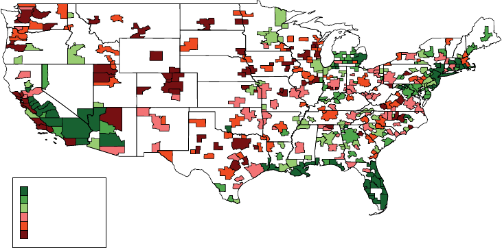
3009
Hurst et al.: regional redistribution
Vol. 106 no. 10
this time period. Using aggregate data published by Fannie/Freddie, we nd that
our dataset includes about one-quarter of the total loans issued by Fannie/Freddie
during the 2007–2009 period. As we discussed above, loans in the Fannie/Freddie
dataset had to meet certain characteristics. Moreover, even after meeting those char-
acteristics, Fannie/Freddie only made a portion of the loans they originated avail-
able online. Given this, and assuming our estimate of Δ r
ˆ
kt
cfactual, GSE
is the same for
GSE loans not in our sample, we scale our estimated transfer number by a factor
of4. Again, this scaling results from the fact that the dollar value of loans originated
in our sample represents one-quarter of the total dollar value of loans originated by
the GSEs during the 2007–2009 period.
Putting all of this together, our back-of-the-envelope estimate suggests that the GSE
constant interest rate policy resulted in direct transfers of $14.5 billion across regions
for loans that were newly originated during the 2007–2009 period. This number
requires little in additional assumptions beyond our baseline empirical strategy, and it
already suggests an economically meaningful role for GSE interest rate policy in gen-
erating cross-region transfers.
25
Again, this back-of-the-envelope calculation misses
many important aspects of the constant interest rate policy, including: (i) equilibrium
effects associated with the response of local income and house prices to changes in
the GSE pricing rule; (ii) equilibrium effects associated with households adjusting
their housing and mortgage behavior in response to changes in the GSE pricing rule;
and (iii) the effect of the policy on loans originated outside of the 2007–2009 period.
More rigorous counterfactual analysis that can address these three issues requires
moving to a structural model of household behavior. We now turn to exactly such
25
We defer a more detailed comparison to other cross-region transfer policies until after presenting our struc-
tural results.
(590,3,000] (53)
(200,590] (52)
(0,200] (53)
(−260,0] (66)
(−495,−260] (66)
[−2,200,−495] (67)
F 4. T MSA, 2007–2009
Notes: This gure shows the average value of transfers Transfer
ikt
PV
for each MSA over the 2007–2009 period.
Positive values represent regions receiving subsidies while negative values represent regions being taxed. See text
for additional description.
3010
THE AMERICAN ECONOMIC REVIEW
OCTObER 2016
a model in order to provide a more comprehensive account of the welfare con-
sequences of the GSEs’ constant interest rate policy. Ultimately, we nd that this
model implies an even more important role for GSE policy in shaping household
welfare than suggested by the $14.5 billion of direct effects at origination.
VI. Consequences of Constant Interest Rates: A Structural Model
In this section, we lay out a quantitative spatial model that captures various
salient factors of the US housing market. We develop a multiregion life-cycle con-
sumption model where households face region-specic shocks to house prices and
labor earnings as well as purely idiosyncratic labor earnings risk. Individuals in
the model can choose whether to own a home or to rent, in addition to choosing
nondurable consumption and liquid savings. Owner-occupied housing is subject to
xed adjustment costs but serves as collateral against which individuals can bor-
row using mortgages. This structural model accounts for endogenous changes in
household behavior in response to changes in mortgage rates and thus can be used
for counterfactual policy analysis. In addition, it allows us to consider the feedback
of local interest rates onto local house prices and local economic activity, which
can potentially have large effects on welfare. The model also allows us to measure
the distributional consequences of the constant interest rate policy for households
with different incomes and ages. This is something we could not explore with the
back-of-the-envelope calculation.
The previous sections have shown that GSE mortgage rates do not respond to
regional shocks. Accordingly, we initially assume that there is no regional variation
in mortgage rates and calibrate the model to match various features of the data. We
then use the model to explore what would happen if the constant interest rate pol-
icy was removed so that mortgage rates vary with local economic conditions in the
manner in which they do in the prime jumbo market documented in the prior part
of the paper.
Our model allows for regional variation in mortgage rates to affect welfare through
three key channels: (i) we assume that households are able to borrow against their
houses subject to holding some minimum equity; (ii) households typically borrow
all but the required down payment when purchasing houses; and (iii) increases in
mortgage rates depress local house prices and economic activity. If interest rates
rise when local conditions deteriorate, the rst channel lowers welfare by making it
more difcult to smooth consumption. The second channel further lowers welfare,
as higher interest rates mean that households in deteriorating regions will delay pur-
chasing housing and reduce the sizes of their eventual purchases. Finally, the third
channel amplies these effects by further driving down economic activity when
interest rates rise. A constant interest rate policy eliminates these effects, and it is in
this sense that the policy transfers resources toward regions experiencing deteriorat-
ing local economic conditions.
A. Model Setup
Demographics and Location.—The economy is characterized by a continuum of
households indexed by i . Household age is indexed by j = 1, . . . , J . Households
3011
Hurst et al.: regional redistribution
Vol. 106 no. 10
enter the labor force at age 25 and retire at age 60. After retirement, households face
stochastic mortality risk with probability of death d
j
. Households live to a maximum
age of 85, so d
85
= 1 .
Households live in specic regions indexed by k , and we assume that house-
holds never move. In our empirical results above, we showed that local economic
conditions such as lagged mortgage default predict current mortgage rates in the
prime jumbo sample but that there is no such relationship in the GSE sample. While
we would want to include various dimensions of regional economic activity in our
model, it is intractable to include all the separate dimensions as separate stochastic
processes. Instead, within our model, we capture various measures of local eco-
nomic conditions in a parsimonious manner by collapsing them into a single sto-
chastic process, γ . We assume that this measure of economic activity ( γ ) in region k
and period t follows the following process:
log γ
k, t
= ρ
γ
log γ
k, t−1
+ ε
k, t
.
In turn, we assume that γ
k, t
affects other local variables such as income and house
prices. The effect of this regional shock γ
k, t
on these other aspects of the model will
be made concrete below as we describe the evolution of income and house prices.
Preferences and Household Choices—Household i receives ow utility
U
ijk
=
(
c
ijk
α
h
ijk
1−α
)
1−σ
___________
1 − σ
from nondurable consumption c
ijk
and housing services h
ijk
.
26
Households discount
expected ow utility over their remaining lifetimes with discount factor β .
Income Shocks.—Time t household labor earnings y for working-age households
are given by
log y
ijk, t
= χ
j
+ z
i, t
+ ϕ
y
γ
k, t
+ ϕ
r
y
ϕ
r
γ
k, t
log z
i, t
= ρ
z
log z
i, t−1
+ η
i, t
,
where χ
j
is a deterministic age prole common to all households, z
i, t
is a purely
idiosyncratic persistent income shock, and ϕ
y
γ
k, t
is a region-specic shock to
income. ϕ
y
is a parameter that governs the sensitivity of household income to the
underlying latent local economic conditions. One symptom of a depressed local
economy will be declines in household income, and this is captured by ϕ
y
. It is
important to include this channel because changes in household income will directly
26
This specication of utility between housing and nondurable consumption is common in the literature. See,
for example, Piazzesi, Schneider, and Tuzel (2007) and Davis and Van Nieuwerburgh (2015). Using data from
the consumer expenditure survey, Aguiar and Hurst (2013) nd that the share of expenditure households allocate
to housing out of total expenditure is roughly invariant with either the level of household income or the level of
household expenditure.
3012
THE AMERICAN ECONOMIC REVIEW
OCTObER 2016
affect the borrowing decisions of households and, as a result, will affect their
response to interest rate variation.
Finally, ϕ
r
y
ϕ
r
γ
k, t
is a term that allows for a feedback multiplier from interest
rates to local income: when interest rates rise, this may depress local economic
activity. As described below, ϕ
r
determines the response of interest rates to local
economic activity, and ϕ
r
y
then determines the response of local income to local
interest rates. Interest rates can directly affect local income through their effects on
local nontradable demand and indirectly through their effects on house prices (see,
e.g., Mian and Su 2014 and Charles, Hurst, and Notowidigdo 2016). As discussed
in our calibration section, we pin down this feedback in the model to match empir-
ical estimates rather than endogenizing local income. In our robustness results we
argue that endogenizing local income would substantially complicate our analysis
with little effect on our conclusions.
When retired, households receive Social Security benets. These benets are
based on lifetime earnings prior to retirement, and they are deterministic until
household death. We describe the computation of these benets in the calibration
section of the model, but they mirror payments under the actual US Social Security
system.
Housing Markets, Mortgages, and Interest Rates.—Housing services can be
obtained from owner-occupied housing or through a rental market. Housing can be
purchased at price p
k, t
=
(
γ
k, t
)
ϕ
h
+ ϕ
r
h
ϕ
r
or rented at price p
k, t
r
f
. We assume that house
prices move exogenously with local economic activity, and ϕ
h
governs the strength
of this correlation. ϕ
r
h
is a term that captures feedback from interest rates to local
house prices in the event that interest rates are not constant ( ϕ
r
> 0 ) . If ϕ
r
h
= 0 ,
then interest rates have no effects on housing prices. We estimate this response empir-
ically rather than endogenizing house prices since this would necessitate modeling
housing supply and dramatically complicate the model. More importantly, we argue
in our robustness results that endogenizing house prices would have little effect on
our conclusions. We denote owner-occupied houses as h
i, t
and rented houses as h
i, t
f
.
Buying or selling an owner-occupied house requires paying a xed cost that is pro-
portional to the current value of the house. That is, the xed fraction lost for house-
hold i when the owners buy or sell their home takes the following form:
F
i, t
=
{
F if h
i, t+1
≠ h
i, t
0 if h
i, t+1
= h
i, t
.
Offsetting the disadvantage that it is costly to adjust one’s housing services, owning
has two benets over renting. First, households can borrow against houses subject
to a minimum equity requirement:
m
ik, t
≤ (1 − θ ) p
k, t
h
i, t
,
where θ is the minimum down payment or equity that must be held in the house.
Second, we assume that the rental stock depreciates at rate δ
f
> δ
h
. This is a
standard assumption that provides a reason that individuals prefer to own rather
3013
Hurst et al.: regional redistribution
Vol. 106 no. 10
than rent. In a competitive equilibrium, the rental price of housing must be equal to
the risk-free rate plus the rate of depreciation of the rental stock:
r
f
= r + δ
f
.
Thus, δ
f
> δ
h
implies that the imputed rental price of owner-occupied housing is
lower than that of renting.
Since the majority of mortgages in the United States have xed rates with an
option to renance, we assume that mortgages in the model take this form. The cur-
rent market interest rate on new mortgages is equal to the risk-free rate plus a risk
adjustment,
r
k, t
m, market
= r + Ψ
k, t
,
where the risk adjustment is declining in regional economic activity:
log Ψ
k, t
= Ψ
–
− ϕ
r
log γ
k, t
.
Ψ
–
is a xed risk adjustment associated with mortgage lending that is constant across
locations. ϕ
r
represents the sensitivity of local mortgage rates to local economic
conditions. In our base specication, we set ϕ
r
= 0 , consistent with the patterns
documented for the GSE loans described above. Our main counterfactuals will be
based on changing ϕ
r
so that it matches the regional variation in response to pre-
dicted local default risk found among the prime jumbo loans.
We assume that households have access to xed rate mortgages, so the current
interest rate that households pay on their mortgages, r
k, t
m, xed
, may differ from the
market rate, r
k, t
m, market
. We assume that when households move houses or purchase
for the rst time, then they must reset their rate so that r
k, t
m, xed
= r
k, t
m, market
. When
not moving, households have the option of keeping their previous xed rate, or re-
nancing to the current market interest rate at cost F
re
, which is proportional to the
value of the house.
27
We extensively discuss the robustness of our results to alterna-
tive mortgage arrangements below.
Finally, in addition to borrowing through mortgages and saving through the pur-
chase of durable housing, households can save in a one-period bond b with risk-free
rate r . We assume that households are otherwise liquidity constrained in that they
can only borrow against the value of their home.
Household Problem.—The household model is solved recursively. Within each
period, households choose whether to move houses, to stay in their initial home, or
to rent. If they stay in their current owner-occupied home, then they must choose
whether to renance. The adjusters include those homeowners who remain home-
owners but change the size of their house, those homeowners who become rent-
ers, and those renters who become homeowners. Conditional on their adjustment
27
The assumption that the renancing cost is proportional to the size of the house simplies computations
under some parameterizations of the xed cost, as discussed below. Also, many of the costs of renancing, like title
insurance, are proportional to home value.
3014
THE AMERICAN ECONOMIC REVIEW
OCTObER 2016
decision, households choose the level of their consumption, their savings in bonds,
and their mortgage debt. For brevity, we leave a formal statement of the value func-
tions to the online Appendix, which also discusses in detail the numerical solution
of the model.
B. Calibration
Our benchmark calibration strategy proceeds in two parts. First, we calibrate
parameters that do not depend on regional economic activity to standard values
from the literature together with standard moments from wealth data. Second, for
parameters that vary with regional activity, we calibrate to match estimates from our
previous empirical results. Our model period is one year, and we calibrate the model
accordingly.
Standard Parameters.—Following Floden and Lindé (2001), we set ρ
z
= 0.91
and σ
η
= 0.21 to match the annual persistence and standard deviation of earnings
in the Panel Study of Income Dynamics (PSID). Their calculation conditions on
education and age and so captures residual earnings risk. Since households in our
model are ex ante identical, this is the relevant empirical object. To calibrate the
life-cycle prole of earnings, χ , we use the age-earnings prole in PSID data esti-
mated by Kaplan and Violante (2010).
During retirement, households receive Social Security benets, which we calcu-
late using the method of Guvenen and Smith (2014). In reality, Social Security ben-
ets are a function of lifetime earnings, but this would substantially complicate the
solution of the model because these lifetime earnings would become a state variable.
However, a relatively accurate measure of lifetime earnings can be imputed from
earnings in the nal period of working life given the persistence of the income pro-
cess. Thus, we forecast lifetime income given income in the nal period of working
and then apply the actual benet ratios from Social Security charts to this imputed
lifetime income.
In addition, following Berger et al. (2015), we capture retirement accounts by
introducing a lump-sum payment at retirement equal to Ω times nal working period
income. This allows us to proxy for the fact that retirement accounts are illiquid
for working-age households but become liquid at retirement. Kaplan and Violante
(2010) argue that it is essential to distinguish between liquid and illiquid wealth in
order to generate realistic marginal propensities to consume, and this payment at
retirement allows us to better capture the life-cycle prole of liquid wealth and so
generate realistic levels of household self-insurance.
As is standard in the risk-sharing literature, we set σ = 2 to generate an inter-
temporal elasticity of substitution of 1/2 . As stated above, our model period is
annual, and we accordingly set the risk-free rate to r = 0.03 to match the average
real one-year Treasury bill rate in the 2000s. In addition, we calibrate an average
risk adjustment ( Ψ
̅
) of 0.01 to match the average real mortgage rate in our data.
We calibrate δ
h
= 0.03 to match the average ratio of residential investment to the
residential stock in Bureau of Economic Analysis (BEA) data. We set θ = 0.20
so that households are required to have a minimum 20 percent down payment. We
pick F = 0.05 so that there is a 5 percent transaction cost from adjusting housing.
3015
Hurst et al.: regional redistribution
Vol. 106 no. 10
This encompasses costs of real estate broker fees, closing costs, and other costs
associated with buying/selling a home. In our baseline results, we assume that
F
re
= 0 . This simplies the problem, as the renancing choice when not mov-
ing will simply deliver r
k, t
m, xed
= min ( r
k, t
m, market
, r
k, t−1
m, xed
) . Below, we discuss the
results for a number of alternatives and show that among these alternatives, this is
the most conservative in terms of generating small implied transfers from the con-
stant interest rate policy.
We jointly pick β, r
f
, Ω , and α to match various wealth and homeownership
targets. We do so under the assumption that ϕ
r
= 0 , which corresponds to the
data-generating process under current policy. To estimate these parameters, we tar-
get a homeownership rate of 69 percent as in the Survey of Consumer Finances
(SCF) data. We also separately target liquid wealth net of all debt relative to income
for working-age and retired households in the SCF.
28
In the SCF data calculation,
we exclude retirement accounts in liquid wealth for working age households and
include retirement accounts in liquid wealth for retired households. Finally, using
BEA data over our sample period, we target a ratio of nonhousing consumption to
residential investment of 15. In our robustness results, we discuss alternative mea-
sures of this expenditure share and argue that our benchmark calibration is con-
servative in its implications: choosing higher housing shares only amplies the
importance of variation in mortgage rates.
We initialize households in the model to match the distribution of income, liquid
wealth net of debt, and housing for 25- to 30-year-old households in the SCF.
29
Together, these targets yield β = 0.916 , r
f
= 0.074 , Ω = 4.13 , and α = 0.88.
Calibrating Regional Variation.—In addition to these relatively standard param-
eters, we must calibrate parameters that vary with regional economic conditions.
Our baseline calibration uses local employment as our measure of economic activity
( γ ). Using annual employment data from the BLS from 1991 to 2013, we esti-
mate an annual AR(1) process for log MSA employment, which yields ρ
γ
= 0.947
and σ
ε
= 0.018.
30
These ndings suggest that shocks to local employment are
somewhat persistent. For simplicity, we assume that local labor earnings move
one-for-one with local employment so that ϕ
y
= 1 , but we assess the importance
of this assumption below in our robustness analysis.
To estimate ϕ
h
, we use house price data from FHFA and regress log MSA
house prices on log MSA employment during the same time period, which
yields ϕ
h
= 0.48. We think of this elasticity as a short- to medium-run adjustment
in house prices. In our baseline analysis, we are abstracting from housing supply
adjustments, which limit the relationship between local employment growth and
house price growth in the long run. However, to account for differential long-run
supply effects, we show the robustness of our results to values of ϕ
h
between zero
28
In the baseline model, only assets net of debt are well dened, so we cannot separately match gross assets
and gross debt in the data.
29
We also assume that the initial distribution of the idiosyncratic and regional income variation matches the
observed cross-sectional distributions for those variables.
30
When estimating the AR(1) process for MSA employment, we remove permanent differences in employment
across MSAs by including MSA xed effects. Likewise, we remove aggregate business cycle effects by including
year xed effects. We include these same xed effects when calculating the elasticity of house prices to local
employment.
3016
THE AMERICAN ECONOMIC REVIEW
OCTObER 2016
and 0.48. A value of ϕ
h
= 0 implies a perfectly elastic housing supply curve even in
the short run in response to local shocks.
We pick the key policy elasticity ϕ
r
so that the regional variation in interest rates
in our model when the GSE pricing policy is removed is consistent with that pre-
dicted by the prime jumbo data described above. In particular, we pick ϕ
r
so that
a two-standard-deviation decrease in γ increases local mortgage rates by 25 basis
points. This is the variation in local mortgage rates to a two-standard-deviation
change in predicted default during the 2007–2009 period for prime jumbo loans
(see Table 5). Given this, the implied elasticity of the total borrowing rate (r + Ψ
–
γ )
to γ is 0.54. We provide robustness results for both larger and smaller ϕ
r
and discuss
alternative counterfactuals in the following section.
Finally, when interest rates decline, this is likely to increase demand for hous-
ing and put upward pressure on house prices as well as on local employment and
earnings, through local multiplier effects. We pin down the strength of these effects
using relatively conservative estimates from VAR evidence on the response of house
prices and GDP to federal funds rate innovations in Christiano, Eichenbaum, and
Evans (1999) and Vargas-Silva (2008). In particular, we calibrate ϕ
r
y
and ϕ
r
h
so that
a 25-basis-point increase in interest rates generates a 0.40 percent decline in house
prices and a 0.20 percent decline in GDP. It is worth noting that both the empirical
and theoretical size of multiplier effects is contentious, but we show below that even
if we conservatively set feedback multipliers to zero, the implied welfare effects of
the constant interest rate policy remain large.
Model Fit.—How well does our model t nontargeted moments? Figure 5 shows
the life-cycle proles in our model compared with the data. Overall the model does
a good job of replicating life-cycle patterns in the data. We match the hump-shaped
prole of nondurable consumption, as well as the increasing homeownership rate as
households age. The model also does a good job of matching the size and life-cycle
prole of total wealth net of debt (which includes the value of the housing stock),
as well as liquid wealth net of debt (which excludes the value of housing from the
measure of wealth). Overall, we think the model provides a close enough t to the
data that we are comfortable using it to assess the counterfactual effects of changes
in GSE interest rate policy.
Our goal is to provide a broad estimate of the impact of the GSE constant inter-
est rate policy on the economy. Household reoptimization in response to changing
policy is a rst-order effect that must be modeled in order to get the impact of this
GSE policy roughly correct. We are less concerned that modest departures between
our model and data along the dimensions above will dramatically affect our broad
policy conclusions.
C. Model Results
To examine the effect of a constant interest rate policy on household well-being,
we simulate household consumption under both the constant interest rate and the
variable interest rate policy. For ease of discussion we label regions with low eco-
nomic activity and high predicted default “bad” (low γ ) regions and regions with
high economic activity and low predicted default “good” (high γ ) regions. We
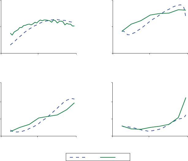
3017
Hurst et al.: regional redistribution
Vol. 106 no. 10
assume that in the absence of intervention from GSEs, mortgage rates would move
with regional economic activity so that good regions would have lower rates and bad
regions would have higher rates. This implies that the constant interest rate policy
will tend to make households in the bad regions better off and households in the
good regions worse off.
To assess the quantitative size of this “transfer” between good and bad regions
under the constant interest rate policy, we ask how much households in a given
region would be willing to pay in units of consumption to change from a variable
interest rate policy to a constant interest rate policy.
31
Formally, let V
j
constant r
( s
jk
) be the indirect utility obtained from solving the house-
hold problem with state s
jk
in a world with ϕ
r
= 0 . Similarly, let V
j
variable r
( s
jk
) be
the indirect utility obtained from solving the model in a world with ϕ
r
> 0, and let
˜
c
jk
and
˜
h
jk
be the choice for nondurable consumption and housing services,
respectively, that obtain this maximal value. Finally, let E
γ, z, j
denote the expectation
31
The online Appendix discusses exactly how we solve the model.
20 40 60
0.5
1
1.5
Panel A. Nondurable consumption
Age
Age
Panel B. Homeownership rate
20 40 60
0
1
2
3
Panel C. Total wealth net of debt Panel D. Liquid wealth net of debt
Model Data
20 40 60
0
0.5
1
Age
Age
20 40 60
−0
0
1
2
F 5. A L-C P: M S D
Note: This gure shows average life-cycle proles generated from the model compared with actual data.
Sources: Nondurable consumption comes from Aguiar and Hurst (2013). Homeownership rates are calculated from
the March CPS, and wealth statistics are calculated from SCF data. Nondurable consumption and total wealth net
of debt are normalized to their life-cycle means. Homeownership rates are unadjusted, and liquid wealth net of debt
is normalized by the mean life-cycle income. See text for additional details.

3018
THE AMERICAN ECONOMIC REVIEW
OCTObER 2016
of these value functions over values of the idiosyncratic shock and age, conditional
on living in a region with economic activity γ .
32
We then solve for λ so that
E
γ, z, j
V
j
constant r
( s
jk
) = E
γ, z, j
variable r
{
U( c
̃
(
1 + λ
)
, h
̃
(
1 + λ
)
) + β E
j
V
j+1
variable r
( s
jk
)
}
.
That is, we compute the one-time percentage change in the consumption aggregate
today that, in expectation, makes households indifferent between being in a world
with constant r
m, market
and a world with variable r
m, market
.
Table 7 shows the implied values of λ for various regions. We discretize the dis-
tribution of γ and focus on regions that had shocks that were one and two standard
deviations above and below the mean region. The rst row expresses the utility gain/
loss ( λ ) from the constant interest rate policy. This is the lifetime consumption gain
as a fraction of today’s consumption. The second row turns the lifetime consumption
equivalent into a dollar amount. To do this, we rst calculate the ratio of consump-
tion to income in the model and then multiply this by median household income in
the United States.
33
This calculation gives that median household consumption is
roughly $42,000. Although this number represents typical consumption per house-
hold, in the model households in bad regions consume less than households in good
regions. This implies that the same λ in a bad region represents a smaller amount
of consumption in dollars than in a good region, so we account for these differ-
ences by using the model’s implied consumption difference across regions to scale
32
In all calculations, unless otherwise noted, we focus on the utility of working-age households since we want
to understand how the mortgage market interacts with household risk. Retired households face no such labor market
risk.
33
We make the conversion from consumption to income in the model since direct measures of consumption in
the data are less reliable than measures of income. The average ratio of consumption to income in the model is 0.85.
The Census Bureau estimates that median household income in 2010 was $49,276. Multiplying the two numbers
implies median consumption of $41,885.
T 7— O-T C E N A R-S R
Regional employment
−2 Standard
deviations
−1 Standard
deviation
0 Standard
deviation
+1 Standard
deviation
+2 Standard
deviations
Baseline
Percent consumption gain
2.26 1.18 −0.02 −1.04 −2.12
Dollar per household effect
No feedback multiplier
$870 $470
−$8 −$457 −$988
Percent consumption gain 1.36 0.70
−0.04 −0.64 −1.26
Dollar per household effect $524 $279
−$17 −$281 −$586
Notes: This table shows the consumption gains estimated from our baseline model. See text for a description of
baseline parameters and the policy experiment. The consumption gain in row 1 is equal to λ × 100, where λ is the
percentage change in consumption that makes a household indifferent between a variable and constant interest rate.
To compute dollar equivalents in row 2, we use the formula (λ × 100) ( λ × 41,885 ×
c
region
_____
c
overall
) where $41,885 is aver-
age household consumption, adjusted for the fact that consumption varies with local economic activity. Baseline
results include both direct interest rate effects as well as indirect feedback effects. The no feedback multiplier results
include only direct effects. Calculations are restricted to working age households subject to labor market risk.
3019
Hurst et al.: regional redistribution
Vol. 106 no. 10
consumption accordingly. The worst regions (on the left side of the table) are made
substantially better off by the constant interest rate policy, while the best regions (on
the right side of the table) are made substantially worse off. Households living in a
region with a two-standard-deviation negative shock to economic conditions would
pay just over 2 percent of today’s consumption to permanently move to a constant
interest rate policy. Conversely, households with a two-standard-deviation positive
shock would pay 2 percent of today’s consumption to avoid the constant interest rate
policy. In terms of dollar values, the constant interest rate policy transfers roughly
$870 per household to the worst regions in Table 7 and taxes the best regions $990.
This represents a one-time net transfer of $1,860 during a period of large regional
dispersion similar to the Great Recession.
This $870 transfer to the most depressed regions (those with a two-standard-
deviation negative shock) is similar in size to the tax rebate checks authorized by the
US Congress during the 2001 and 2008 recessions, which were also one-time pay-
ments during recessions (which ranged from $500 to $1,000 per qualifying house-
hold). However, it is important to note that our $870 transfer converts the expected
lifetime effects of the constant interest rate policy into a single one-time transfer
equivalent. Since tax rebates have now become a common tool for ghting reces-
sions, the present discounted value of future tax rebates is most likely higher than
the size of any one rebate check. The other difference is that the transfer provided
via the constant interest rate mortgage policy is funded by “taxing” the regions that
are doing relatively well by roughly the same amount. While one might think the
regions that are doing relatively well could borrow from private lenders to avoid
this tax, it is important to remember that this is prevented by the GSEs’ overall cost
advantage, as noted in Section II.
Rather than focusing on implicit transfers from regions with particular employ-
ment shocks, we can also calculate the total resources transferred from all regions
with positive employment shocks to all regions with negative employment shocks.
34
The average household in a location with a negative regional employment shock
values the constant interest rate policy equivalently to a one-time $350 payment.
At the same time, the average household in a location with a positive employment
shock would be willing to make a one-time payment of $465 to move permanently
to a variable interest rate policy. Thus, the total implicit net transfer implied by the
constant interest rate policy averages $815 per household. The aggregate value of
the transfers induced by the constant interest rate policy comes to $47 billion.
35
It is important to note that this $47 billion should be interpreted as a one-time
equivalent of the total discounted lifetime transfers across regions. For comparison,
the Department of Labor forecasts that total unemployment insurance (UI) benets
paid in 2014 alone will equal roughly $50 billion. Thus, transfers through the con-
stant interest rate policy are smaller than the large-scale social insurance arising
34
To compute this average transfer, we compute
∫
γ<0
f (γ )
(
1 + λ
(
γ
)
)
dγ and
∫
γ>0
f (γ )
(
1 + λ
(
γ
)
)
dγ, where
f(γ ) is the probability of experiencing a given γ shock and λ
(
γ
)
is the welfare evaluation of a constant interest rate
policy for a household living in a region with that γ . To provide a better approximation to f (γ ) we expand the γ grid
from 5 to 15 points for this calculation, but we nd nearly identical results when using 5 points.
35
This value is equal to $350 × 115/2 + $465 × 115/2 million households. We divide by 2 because one-half
of the households in our model live in regions that get positive shocks, while the other half live in regions that get
negative shocks.
3020
THE AMERICAN ECONOMIC REVIEW
OCTObER 2016
from UI, but are certainly large enough to warrant substantial attention. Our results
imply large transfer payments across regions so that the constant interest rate policy
has signicant redistributional consequences.
The direct effect of abandoning the constant interest rate policy is that interest
rates will then rise when economic activity deteriorates. This directly reduces wel-
fare for anyone who will renance during the period when economic conditions
remain depressed, since it makes it more difcult to smooth consumption through
home equity loans and also reduces the affordability of housing.
36
In our baseline
model, we also allow for local multipliers so that increases in mortgage rates further
depress local house prices and economic activity. This amplies the direct effects
of higher interest rates for households that renance but also lowers utility even
for households that never plan to renance. What are the relative contributions of
direct versus indirect multiplier effects? In the third and fourth rows of Table 7 we
set ϕ
r
h
= ϕ
r
y
= 0 and recompute the size of transfers when local multipliers are set
to zero. These rows show that direct interest rate effects account for about 60 percent
of the transfers from the constant interest rate policy.
It is also useful to relate these full model results to the back-of-the-envelope
results from the previous section. In that section, we showed that when ignoring
indirect feedback effects and household reoptimization and focusing only on orig-
inations rather than on all loans, we arrived at an already substantial transfer of
roughly $15 billion. Our structural model shows that when accounting for all of
these missing effects, implied transfers rise to an even more substantial $47 bil-
lion. Around 40 percent of this increase comes from indirect multiplier effects on
local income and house prices, which are not captured by the back-of-the-envelope
calculation. If we turn off the indirect multiplier effects in the model, transfers fall
to just over $28 billion. The general equilibrium effects of the interest rate policy
on local house prices and therefore local income thus accounts for a substantial
portion of the reason why our model is yielding transfers larger than our back of
the envelope calculation. The remainder of the difference arises from the fact that
the model measures the welfare consequences of the GSE policy for all households
rather than just those adjusting their mortgages in a given year and also accounts
for household reoptimization. Clearly, the back-of-the-envelope numbers and those
from the model are not identical, and including effects that cannot be captured in
the simple reduced-form exercise amplies our conclusions. Nevertheless, the fact
that the overall order of magnitude of welfare consequences is similar between the
back-of-the-envelope calculation and the model provides some reassurance that our
model does not produce implausible results.
Our model also allows us to assess the effects of the policy across different sub-
groups of the population. We choose to focus on two dimensions of heterogene-
ity: age and income. Table 8 shows the constant interest rate policy has the largest
effects on middle-income, middle-aged households. In our model, the importance of
mortgage rates for household welfare depends on the level of their mortgage debt,
and this is closely tied to age and income. The model implies that the GSE pric-
ing policy has a much larger effect on middle-aged households relative to younger
36
Households who do not renance will also be affected due to the dynamic nature of the problem: changes in
interest rates will affect the value of renancing in the future and thus household continuation values.

3021
Hurst et al.: regional redistribution
Vol. 106 no. 10
households because the young mostly choose to rent and are thus less sensitive to
the local mortgage rate. Similarly, the implied transfer is largest for middle-income
households within each region, as the poorest households do not own houses, while
the richest households have little mortgage debt. Thus, not only are there important
transfers at the regional level, there is also important variation in these transfers
across subgroups. Our model suggests that in many ways the GSE constant interest
rate policy distributes large amounts of resources within middle-class households.
All of our results so far (in Tables 7 and 8) focus on the ex post redistributional
consequences of the GSE pricing rule, because this makes our results more com-
parable to existing studies of scal transfers. For example, studies of state transfers
arising from the federal income tax system focus on the transfers from states with
high income to those with low income rather than on the ex ante consequences of
the tax system behind the “veil of ignorance.” Similarly, studies of unemployment
benets often look at the effects on individuals who actually become unemployed
rather than their ex ante consequences for utility. Nevertheless, it is straightforward
to calculate the ex ante welfare effects of the GSE constant interest rate policy.
With concave utility, if the variable interest rate resulted in a pure mean preserving
spread in consumption, it would necessarily lower ex ante welfare. We nd that in
our benchmark results, the ex ante lifetime consumption equivalent is neverthe-
less very small: households would pay only 0.1 percent of current consumption to
move from the variable to the constant interest rate policy. Part of the reason for
the small welfare effects is that in general the costs of business cycles are quite
small (a point made in Lucas 1987). The welfare costs of the regional business
cycles in our model are slightly higher because the regional shocks we estimate are
more persistent than the shocks typically estimated for aggregate business cycles.
Despite having relatively small ex ante welfare gains, our model predicts large
ex post transfers across regions. These results are robust to various changes in our
parameter specication.
T 8— O-T C E N A R-S R,
A I (Percent)
Regional employment
Consumption gain
−2
Standard
deviations
−1
Standard
deviation
0
Standard
deviation
+1
Standard
deviation
+2
Standard
deviations
Overall 2.26 1.18
−0.02 −1.04 −2.12
Young 1.76 1.02
−0.08 −0.90 −1.98
Middle-aged
Low-income
Middle-income
High-income
2.50
1.46
2.64
2.18
1.26
0.76
1.36
1.22
0.00
−0.06
−0.02
0.04
−1.14
−0.82
−1.16
−0.92
−2.18
−1.74
−2.32
−1.60
Notes: This table shows the consumption gains estimated from our baseline model, by age and income. See text
for a description of baseline parameters and the policy experiment. The consumption gain in each row is equal to
λ × 100, where λ is the percentage change in consumption that makes a household indifferent between a variable
and constant interest rate. Calculations are restricted to working-age households subject to labor market risk. We
dene “young” as households of ages 25–34 and “middle-aged” as households of ages 35–59. Income groups are
split into the highest one-third, middle one-third, and lowest one-third of the stochastic income process for work-
ing households.

3022
THE AMERICAN ECONOMIC REVIEW
OCTObER 2016
D. Robustness and Model Discussion
Sensitivity of Results to ϕ
r
.—In our benchmark calibration, we pick ϕ
r
to match the
variation in interest rates observed in the jumbo market during the Great Recession.
However, if the jumbo market piggybacks off of the GSE policy in picking interest
rates, the true sensitivity might be larger than what we nd in the data. Conversely,
our empirical section controlled for various observables around the conforming
threshold and argued that observable default varies smoothly across the threshold.
However, if borrowers just above the conforming threshold were instead riskier than
borrowers just below the threshold, then our benchmark estimates of ϕ
r
might be
overstated. Table 9 shows implied transfers under various values of ϕ
r
. In particular,
we target a 35-basis-point variation in response to a two-standard-deviation regional
shock (referred to as “larger variation”) and then separately a 15-basis-point varia-
tion in response to a two-standard-deviation regional shock (referred to as “smaller
variation”). Unsurprisingly, the level of implied transfers is increasing in ϕ
r
.
Increasing the variation by 10 basis points in response to a two-standard-deviation
change in local economic activity increases the total transfers from good to bad
regions by about 50 percent relative to the base specication. Cutting the variation
by 10 basis points in response to a two-standard-deviation change in local economic
activity reduces the total transfer from good to bad regions by about 50 percent.
The key point is that even with a much smaller value of ϕ
r
(compared with what we
estimate from the prime jumbo data), the transfers from good regions to bad regions
through the constant interest rate policy remain quite large.
Alternative Mortgage Contracts.—In our baseline model, we make many assump-
tions surrounding the mortgage contracts available to households. In particular, we
assume that all mortgages are xed rate, that households can adjust their mortgage
balances without resetting the rate on their mortgage, and that households can re-
nance to a different mortgage rate without paying a cost. These assumptions capture
many realistic aspects of mortgage contracts but at the same time make some sim-
plications in order to increase the tractability of the model solution. For example,
most mortgages in the United States are xed rate. Additionally, most households
can reduce their mortgage balance (by making extra payments) without paying any
T 9—S D V ϕ
r
(Percent)
Regional employment
−2
Standard
deviations
−1
Standard
deviation
0
Standard
deviation
+1
Standard
deviation
+2
Standard
deviations
Consumption gain: benchmark (25 bp)
2.26 1.18
−0.02 −1.04 −2.12
Larger variation (35 bp)
3.16 1.56
−0.05 −1.50 −2.63
Smaller variation (15 bp)
1.39 0.74 0.00
−0.67 −1.32
Notes: This table shows the robustness of our estimated consumption gains to different interest rate sensitivities to
local economic conditions. See text for a description of baseline parameters and the policy experiment. The con-
sumption gain in each row is equal to λ × 100, where λ is the percentage change in consumption that makes a
household indifferent between a variable and constant interest rate. We alter the value of ϕ
r
such that the benchmark
variation in regional employment produces alternative variability in mortgage rates.
3023
Hurst et al.: regional redistribution
Vol. 106 no. 10
renancing costs. However, households typically have to pay a renancing cost to
increase mortgage balances (if they do not have a home equity line of credit) or to
reset their rate. Several of these assumptions simplify the solution of the model sub-
stantially, but how important are they for our conclusions?
In the online Appendix, we explore the sensitivity of our results to changing the
mortgage contracts available to households within the model. In particular, we rst
explore a version of the model where we assume variable rather than xed-rate
mortgages (i.e., the mortgage rate paid by a household in period t is always equal
to r
k, t
m, market
.) Next, we allow for costly renancing by forcing households to pay a
xed cost, F
re
every time they renance. Finally, we solve a version of a much more
complicated model with xed-rate, xed-balance mortgages, and costly renanc-
ing. The details of these robustness exercises can be found in the online Appendix.
Importantly, we nd the size of cross-region transfers is quantitatively similar
across all these alternative specications. From this, we conclude that our results
are not dependent on the type of mortgage contract we choose to model in our base
specication.
It might seem surprising that moving from xed to variable interest rates has little
effect on our conclusions. This occurs because most households are largely making
their decisions based on life-cycle considerations and idiosyncratic factors rather
than timing purchases or delaying purchases to take advantage of low rates. When
combined with persistent regional shocks, this means that most households end up
having a xed rate mortgage which is equal to or very close to the prevailing inter-
est rate so that the distinction between xed and adjustable rates is not particularly
important. Put differently, for realistic prepayment rates, local economic conditions
are much more persistent than the average life of a mortgage.
37
Modeling Default.—In our results thus far, we do not explicitly model household
default decisions and instead capture the effects of local conditions on credit risk
and interest rates through their effects on the risk adjustment factor ( Ψ ). While it
would be desirable to build a model with endogenous credit risk and interest rates
rather than exogenously linking these variables to local conditions, this would also
substantially complicate the model. To what extent would such a model change any
of our conclusions? Since we are interested in evaluating the effects of a change
in interest rate policy, the main way in which endogenizing default could matter
would be if default responds strongly to interest rates. These responses might then
alter the size of implied transfers. For example, if defaults also rise with interest
rates, then abandoning the constant interest rate policy would further increase the
response of default risk and interest rates to local conditions, which would amplify
our conclusions.
While a full-edged model of strategic default with endogenous interest rates is
beyond the scope of this paper, it is straightforward to provide some sense of the
sensitivity of our results along this dimension. In the online Appendix, we amend
our model by endogenizing default using a simple version of Campbell and Cocco
(2015). Reassuringly, this model suggests that our results are unlikely to be altered
37
In our baseline model, prepayment rates are just under 14 percent which is roughly in line with the annual
prepayment rate of 9–12 percent in our data.
3024
THE AMERICAN ECONOMIC REVIEW
OCTObER 2016
by explicitly modeling local credit risk and endogenous interest rates. This is because
in this extended model, default barely responds to local interest rate variation: a
one-standard-deviation ( cross-MSA) increase in interest rates only increases default
by 0.027 ( cross-MSA) standard deviations.
38
Applying our estimates from the rst
half of the paper, this increase in expected default should lead to only an additional
1. 1-basis-point-increase in interest rates.
39
This would increase the size of implied
transfers, but in a fairly negligible way that is well within the range of robustness
we considered in Table 9. Thus, we conclude that formally modeling default and
endogenous interest rates will greatly complicate our model without substantively
altering its quantitative implications.
Labor Mobility.—Our base assumption is that labor is immobile across regions.
One way to support a regional equilibrium is by allowing factors to move across
regions. Two facts make us believe that allowing for such mobility would not alter
our results in any meaningful way. First, we estimate our regional income processes
on actual data. The underlying data takes into account both the true underlying pro-
cess driving the regional shocks to income as well as any endogenous response
of factors across regions. Our approach cannot distinguish between large regional
shocks that are mitigated in part through factor mobility and slightly smaller shocks
in a world with less factor mobility. Given that we are using these processes to cali-
brate our model, any migration that actually occurs will be captured in our estimates.
Second, there is a large literature showing that permanent regional shocks lead to
sizable migration responses (see, for example, Blanchard and Katz 1992). There is
less evidence that regional migration is important in response to the kinds of tempo-
rary regional shocks captured by our model. With costly migration, individuals may
choose to ride out the regional business cycle as opposed to paying the migration
cost and moving to another region. In fact, there was very little net migration from
regions hit hard during the most recent recession to regions that were hit less hard
(see Yagan 2016). For these reasons, we believe that abstracting from migration will
not signicantly change the model’s main results.
Endogenous Income and House Prices.—In our baseline model, we allow for
feedback from interest rates to local house prices and income that is consistent
with observed relationships in the data. However, we do not endogenize this feed-
back, since this would add numerous layers of complication to an already complex
model.
40
Ultimately, the parameters of this more complicated model would need
to be picked so as to match empirical relationships between interest rates, income,
and house prices. For tractability, we instead skip this intermediate step and match
empirical relationships directly.
38
In particular, a one-standard-deviation increase in interest rates (12.5 basis points) in the model increases
default from 2.58 percent to 2.66 percent. Dividing this 0.08 percent change by the 2.9 percent cross-MSA standard
deviation in the last row of Table 1 delivers the 0. 027-standard-deviation change in default.
39
A 1 percent increase in predicted default implies that interest rates should rise by 13.48 basis points
( 0.08 × 13.48 = 1.07 basis points).
40
For example, we would have to take a stand on the importance of nominal frictions, elasticity of housing sup-
ply, share of tradables in local employment, and capital and labor mobility. This would also introduce one or more
additional state variables and require forecasting and solving for equilibrium.
3025
Hurst et al.: regional redistribution
Vol. 106 no. 10
This could potentially be problematic if the historical relationship between
income, house prices, and interest rates would change if the GSE constant interest
rate policy was altered. However, this is unlikely to be the case: we are not consid-
ering the elimination of the GSEs, which would have large macroeconomic effects
on housing markets. Instead we consider a simple change in the pricing of local
risk, which is already present for the private segment of the market. Furthermore,
in the online Appendix, we show that our results are insensitive to the overall level
of variation in house prices and income. In addition, in the model, housing demand
falls only mildly in response to a 25-basis-point increase in interest rates, so that
we would not expect any equilibrium effects from changes in GSE interest rate
policy to be dramatic or alter historical relationships. Put differently, we believe we
have shown that the constant interest rate policy plays an important role in redis-
tributing resources across regions. However, it is unlikely that the introduction of
25-basis-point variation in interest rates would generate systemic aggregate effects
or change the overall institutional structure of housing markets in a way that would
invalidate our modeling strategy.
Additional Robustness.—Finally, in the online Appendix, we explore the robust-
ness of our model results to changes in a variety of other model parameters and
calibration targets. For example, we explore the sensitivity of our results to changes
in both ϕ
y
and ϕ
h
as well as to changes in housing adjustment costs, the calibration
of wealth, and housing expenditure shares. As we show, these parameters have little
effect on the level of cross-region transfers, and if anything our baseline calibration
is relatively conservative.
VII. Conclusion
Recent business cycles have yielded dramatic disparities in regional outcomes
within the United States. While prior research has carefully studied the role of tax and
transfer systems in mitigating local shocks, we propose an entirely different mecha-
nism through which federal policy may provide some regional redistribution. In this
paper we empirically document the extent to which local mortgage rates (do not)
vary with local economic conditions. The United States is unique in the extensive
role that government institutions play in the mortgage market. In 2008, when placed
into conservatorship, the Federal National Mortgage Association (Fannie Mae) and
the Federal Home Loan Mortgage Corporation (Freddie Mac) owned or guaranteed
roughly one-half of the $12 trillion US mortgage market. We establish empirically
that, despite large regional variation in predictable default risk, there is essentially
no spatial variation in GSE mortgage rates (conditional on borrower observables).
In contrast, we show that mortgage rates in the private “prime jumbo” market, where
loans are larger than the conforming limit but comparable on many dimensions to
loans backed by the GSEs, were strongly correlated with ex ante predicted default
probabilities across geography. Using a structural spatial model of collateralized
borrowing where households face both idiosyncratic and region-specic shocks,
we estimate the magnitude of transfers across regions when interest rates are set
using a constant national rate rather than in response to local risk. Overall transfers
are large, and for the regions hit with particularly bad shocks, they are comparable
3026
THE AMERICAN ECONOMIC REVIEW
OCTObER 2016
in size to recent scal stimulus programs such as tax rebates and unemployment
insurance.
Although a range of consequences to the housing and mortgage markets are
often attributed to the presence of Fannie Mae and Freddie Mac, their common
national interest rate policy is one important and understudied dimension of their
impact on households’ choices. By distributing resources across US regions in a
state-contingent way, in addition to providing countercyclical liquidity to the mort-
gage market, Fannie Mae and Freddie Mac provide meaningful insurance during
aggregate downturns. It is worth noting that, so long as the current structure of GSEs
persists, we expect this resource redistribution to continue since their lower cost of
funds—attributed to both the implicit too-big-to-fail guarantee and their scale—
makes it difcult for the private market to undo any potential mispricing by the
GSEs. In particular, if political constraints prevent the GSEs from raising interest
rates in declining markets and lowering interest rates in relatively strong markets,
the cost differential prevents private markets from competing with lower interest
rates in relatively stronger markets. We hope to better understand the impact of the
current structure of GSEs and in particular the constant rate policy on housing mar-
ket activity and house prices in future work.
We conclude by noting two important caveats of our result. Throughout the anal-
ysis, our benchmark for how much mortgage rates should vary with ex ante default
probabilities in the GSE market is the variation we observe in our sample of prime
jumbo loans. We feel this is a good comparison group, particularly when we match
on factors like MSA, FICO score, LTV ratio, documentation type, xed-rate, and
30-year term. However, we realize that even in private markets, political economy
considerations may still limit the extent to which interest rates can vary spatially.
Additionally, discussions with securitizers of private mortgages suggest that they
often attempt to use the same mortgage pricing platforms as the GSEs to increase
their pricing models’ transparency for secondary market investors. Both of these
factors may lead us to understate the spatial variation we would observe in the mort-
gage market if GSEs fully priced local default probabilities. These factors would
in turn imply that our estimates of state-contingent transfers across regions will
be a lower bound on the true extent of transfers. It is worth noting, however, that
using our model, we recomputed transfers under a number of alternative assump-
tions about how mortgage rates would vary with local predicted default probabilities
across regions and continued to nd large implied transfers.
Additionally, we want to stress that we are not saying the GSE policy is the
optimal way to transfer resources across regions in state-contingent ways. Many
have argued for the potential welfare-reducing role of the GSEs in distorting the
allocation of capital (see, e.g., Elenev, Landvoigt, and Van Nieuwerburgh 2016).
Moreover, policy makers have many other tools to transfer resources across regions
if they so desire. Our goal in this paper is to study the impact of a current policy as
opposed to providing either a full welfare analysis of the existence of the GSEs or
discussing the optimal way to transfer resources across regions.
3027
Hurst et al.: regional redistribution
Vol. 106 no. 10
REFERENCES
Agarwal, Sumit, Gene Amromin, Itzhak Ben-David, Souphala Chomsisengphet, Tomasz Piskorski,
and Amit Seru.
2012. “Policy Intervention in Debt Renegotiation: Evidence from the Home Afford-
able Modication Program.” NBER Working Paper 18311.
Aguiar, Mark, and Erik Hurst. 2013. “Deconstructing Life Cycle Expenditure.” Journal of Political
Economy 121 (3): 437–92.
Asdrubali, Pierfederico, Bent E. Sorensen, and Oved Yosha. 1996. “Channels of Interstate Risk Shar-
ing: United States 1963–1990. Quarterly Journal of Economics 111 (4): 1081–1110.
Beraja, Martin, Erik Hurst, and Juan Ospina. 2016. “The Aggregate Implications of Regional Busi-
ness Cycles.” NBER Working Paper 21956.
Berger, David, Veronica Guerrieri, Guido Lorenzoni, and Joseph Vavra. 2015. “House Prices and Con-
sumer Spending.” NBER Working Paper 21667.
Blanchard, Olivier Jean, and Lawrence F. Katz. 1992. “Regional Evolutions.” Brookings Papers on
Economic Activity (1): 1–75.
Campbell, John Y., and João Cocco. 2015. “A Model of Mortgage Default.” Journal of Finance 70 (4):
1495–1554.
Charles, Kerwin Ko, Erik Hurst, and Matthew J. Notowidigdo. 2016. “The Masking of the Decline
in Manufacturing Employment by the Housing Bubble.” Journal of Economic Perspectives 30 (2):
179–200.
Christiano, Lawrence J., Martin Eichenbaum, and Charles L. Evans. 1999. “Monetary Policy Shocks:
What Have We Learned and to What End?” In Handbook of Macroeconomics, Vol. 1A, edited by
John B. Taylor and Michael Woodford, 65–148. New York: Elsevier.
Davis, Morris A., and Stijn Van Nieuwerburgh. 2015. “Housing, Finance, and the Macroeconomy.” In
Handbook of Urban and Regional Economics, Vol. 5, edited by Gilles Duranton, J. Vernon Hender-
son, and William C. Strange, 753–811. New York: Elsevier.
Di Maggio, Marco, Amir Kermani, and Rodney Ramcharan. 2015. “Monetary Pass-Through:
Household Consumption and Voluntary Deleveraging.” https://www0.gsb.columbia.edu/faculty/
mdimaggio/papers/dimaggio_kermani_ramcharan_feb25.pdf.
Elenev, Vadim, Tim Landvoigt, and Stijn Van Nieuwerburgh. 2016. “Phasing out the GSEs.” Journal
of Monetary Economics 81: 111–32.
Farhi, Emmanuel, and Iván Werning. 2012. “Fiscal Unions.” NBER Working Paper 18280.
Farhi, Emmanuel, and Iván Werning. 2014. “Labor Mobility within Currency Unions.” NBER Work-
ing Paper 20105.
Feyrer, James, and Bruce Sacerdote. 2011. “Did the Stimulus Stimulate? Real Time Estimates of the
Effects of the American Recovery and Reinvestment Act.” NBER Working Paper 16759.
Finkelstein, Amy, and James Poterba. 2014. “Testing for Asymmetric Information Using ‘Unused
Observables’ in Insurance Markets: Evidence from the UK Annuity Market.” Journal of Risk and
Insurance 81 (4): 709–34.
Floden, Martin, and Jesper Lindé. 2001. “Idiosyncratic Risk in the United States and Sweden: Is There
a Role for Government Insurance?” Review of Economic Dynamics 4 (2): 406–37.
Guvenen, Fatih, and Anthony Smith. 2014. “Inferring Labor Income Risk and Partial Insurance from
Economic Choices.” Econometrica 82 (6): 2085–2129.
Hurst, Erik, Benjamin Keys, Amit Seru, and Joseph Vavra. 2016. “Regional Redistribution through
the US Mortgage Market: Dataset.” American Economic Review. http://dx.doi.org/10.1257/
aer.20151052.
Kaplan, Greg, and Giovanni L. Violante. 2010. “How Much Consumption Insurance beyond
Self-Insurance?” American Economic Journal: Macroeconomics 2 (4): 53–87.
Keys, Benjamin J., Tomasz Piskorski, Amit Seru, and Vikrant Vig. 2013. “Mortgage Financing in the
Housing Boom and Bust.” In Housing and the Financial Crisis, edited by Edward L. Glaeser and
Todd Sinai, 143–205. Chicago: University of Chicago Press.
Keys, Benjamin J., Tomasz Piskorski, Amit Seru, and Vincent Yao. 2014. “Mortgage Rates, Household
Balance Sheets, and the Real Economy.” NBER Working Paper 20561.
Lehnert, Andreas, Wayne Passmore, and Shane M. Sherlund. 2008. “GSEs, Mortgage Rates, and Sec-
ondary Market Activities.” Journal of Real Estate Finance and Economics 36 (3): 343–63.
Lucas, Deborah, and David Torregrosa. 2010. “Fannie Mae, Freddie Mac, and the Federal Role in the
Secondary Mortgage Market.” Washington, DC: Congressional Budget Ofce Study.
Lucas, Robert E. 1987. Models of Business Cycles. Jahnsson Lectures. Oxford: Blackwell.
Lustig, Hanno N., and Stijn Van Nieuwerburgh. 2005. “Housing Collateral, Consumption Insurance,
and Risk Premia: An Empirical Perspective.” Journal of Finance 60 (3): 1167–1219.
3028
THE AMERICAN ECONOMIC REVIEW
OCTObER 2016
Lustig, Hanno, and Stijn Van Nieuwerburgh. 2010. “How Much Does Household Collateral Constrain
Regional Risk Sharing?” Review of Economic Dynamics 13 (2): 265–94.
Mayer, Christopher, Karen Pence, and Shane M. Sherlund. 2009. “The Rise in Mortgage Defaults.”
Journal of Economic Perspectives 23 (1): 27–50.
Mian, Atif, Kamalesh Rao, and Amir Su. 2013. “Household Balance Sheets, Consumption, and the
Economic Slump.” Quarterly Journal of Economics 128 (4): 1687–1726.
Mian, Atif, and Amir Su. 2014. “What Explains the 2007–2009 Drop in Employment?” Economet-
rica 82 (6): 2197–2223.
Mian, Atif, Amir Su, and Francesco Trebbi. 2015. “Foreclosures, House Prices, and the Real Econ-
omy.” Journal of Finance 70 (6): 2587–2634.
Nakamura, Emi, and Jón Steinsson. 2014. “Fiscal Stimulus in a Monetary Union: Evidence from US
Regions.” American Economic Review 104 (3): 753–92.
Piazzesi, Monika, Martin Schneider, and Selale Tuzel. 2007. “Housing, Consumption, and Asset Pric-
ing.” Journal of Financial Economics 83 (3): 531–69
Sala-i-Martin, Xavier, and Jeffrey Sachs. 1991. “Fiscal Federalism and Optimum Currency Areas: Evi-
dence for Europe from the United States.” NBER Working Paper 3855.
Scharfstein, David S., and Adi Sunderam. 2013. “Concentration in Mortgage Lending, Renancing
Activity and Mortgage Rates.” NBER Working Paper 19156.
Sherlund, Shane. 2008. “The Jumbo-Conforming Spread: A Semi-Parametric Approach.” Federal
Reserve Board of Governors Finance and Economics Discussion Series Working Paper 2008-01.
Vargas-Silva, Carlos. 2008. “Monetary Policy and the US Housing Market: A VAR Analysis Imposing
Sign Restrictions.” Journal of Macroeconomics 30 (3): 977–90.
Yagan, Danny. 2016. “Is the Great Recession Really Over? Longitudinal Evidence of Enduring
Employment Impacts.” http://eml.berkeley.edu/~yagan/EnduringImpact.pdf (accessed August 30,
2016).
Zidar, Owen. 2015. “Tax Cuts for Whom? Heterogeneous Effects of Income Tax Changes on Growth
and Employment.” NBER Working Paper 21035.
