Pivot tables for call detail records analysis

2012

POLICE TECHNICAL

Aaron Edens

PIVOT TABLES FOR CALL

DETAIL RECORDS ANALYSIS

Pivot Tables for Call Detail Record Analysis

Pivot tables are a powerful function built into Microsoft Excel which can be used to translate call detail

records (CDRs) into something useable.

Remember: NEVER WORK WITH YOUR ORIGINAL DATA! You should only use a copy of the files and

not the originals you received from the cellular service provider.

Step 1-Clean Your Data

In order for a pivot table to work effectively the call detail record data must be standardized. Some

cellular service providers include routing codes, extra digits, and additional information in the same

text box as the phone number. These extra digits will need to be cleaned from the data. You may also

see additional data in the Dialed Number column which does not reflect an actual phone call such as

the case when someone only enters a partial or incomplete phone number before pressing the send

button. As those are not actual calls, but merely records of incomplete calls I delete those records.

Depending on the provider you may also see extra routing numbers or extra digits, such as *67 when

someone blocks their phone number from appearing on caller ID. There are a number of methods for

removing those leading digits including the Find and Select function from the Home tab of Excel.

However, after much trial and error I have become a faithful user of a free suite of tools called ASAP

Utilities. These tools make it very easy to format all of your data quickly.

You may also note that Excel interprets some or all of your data contained in call detail records as text

and not as numbers. When Excel detects numbers stored as text is places a small green triangle in the

upper left of the cell.

You could click on the green triangle and manually change each cell of text into a number but that

would take forever.

To quickly convert all text to numbers highlight the entire column by clicking the cell with a letter in it

at the top of the column. Right click and select Format Cells.

Select Number. By default you will see the number 2 in the box marked Decimal Places. Change that

to 0.

Step 2-Insert New Columns

If you call detail records do not have a separate column for the target phone number you will need to

create one. The easiest way is to right click you mouse button on the column header A and select

Insert. This will automatically insert a column and shift the data over. In the A1 cell type something to

help you remember what this data is such as Target Number. This will be important later as there will

be multiple columns to choose from and you want to make sure you select the proper one.

Insert the target number and then fill the entire column with your target telephone number. The

easiest way to do this is to copy the phone number three times into the first three cells. Then highlight

all three cells by left clicking you mouse button and dragging it downwards until all three cell are

highlighted. If you hover your mouse cursor over the lower right corner of the last cell what looks like a

small plus sign + will appear. Left click the plus sign + and Excel will automatically populate all of the

cells below it with the target number.

You are also going to need to insert another column for your Other Numbers. This data already exists

in the call detail records but some providers display this information in multiple different columns.

Right click you mouse button and select Insert again to place a new blank column in your data and label

it with something you will remember such as Other Number. The other phone numbers need to be

consolidated in one column. Depending on the provider, you may have to sort your data by the

Direction of the call or the Caller ID column to obtain this information. Copy the data from those rows

into your new column so that all of the other phone numbers are in one place.

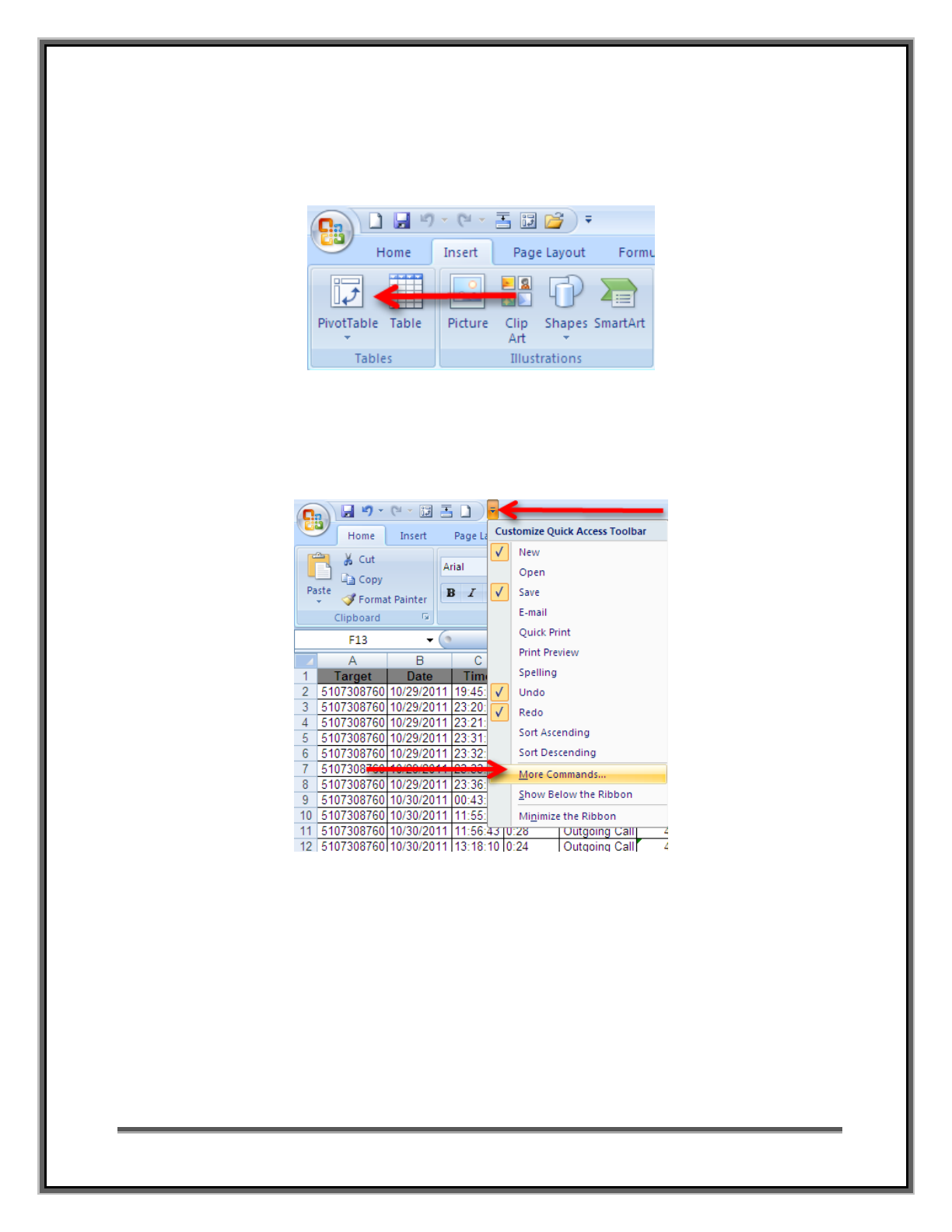
Step 3-Finding the Pivot Table

The Pivot Table function is located in two places in Excel. The first in the Insert tab located at the top

of the Excel workbook.

You may also wish to add the Pivot Table to the Quick Access Toolbar located at the upper left corner

of the Excel workbook. In order to add the Pivot Table to the toolbar, select the drop down error to the

right of the toolbar. You will need to select More Commands to locate the Pivot Table function.

Next select All Commands and scroll down until you see the Pivot Table Wizard. Select the Add button

to include the Pivot Table Wizard in the toolbar.

When you are done you should see this icon in your Quick Launch Toolbar.

Step 4-Using the Pivot Table Wizard

Select Pivot Table from either the Insert Tab or the newly created icon the Quick Launch Toolbar. This

will start the program and automatically bring up this screen:

We are not going to do anything fancy from this screen so select Next. You could select Finish from this

screen but there are some different options in the following steps.

The Step 2 screen tells the Pivot Table Wizard where the data is going to come from.

Before selecting next make sure all of the data in your sheet is selected. The data in the sheet should be

surrounded by a moving row of dashes sometimes referred to as ‘marching ants’.

All of the data inside the highlighted area and surrounded by the marching ants is going to be imported

into the Pivot Table. If for some reason all of the data is not selected, or if the entire work sheet is

highlighted including columns and rows with no data in it, select cancel and click on any cell containing

data on the sheet and re-run the Pivot Table Wizard.

To complete the setup of the Pivot Table select the finish button from the Step 3 screen. By default this

will create the Pivot Table in a new worksheet which will be added in front of your existing worksheets.

Step 5-Using the Pivot Table

Once the Pivot Table process has been completed you should be presented with the following in a new

sheet added to your Excel workbook:

All of the column headers, including the Target Number and Other Number should appear in the Pivot

Table Field List located in the upper right of the screen. From this screen you can perform basic call

frequency analysis using the data from the call detail records.

Select Target Number and Other Number by placing a check mark in the boxes. You data may appear in

the boxes labeled Row Labels and Values. If the data is not automatically in those boxes, click and drag

the data so it appears as below:

Sometimes the data in the Values box will be different and will say Sum of Target and not Count of

Target. If this happens you will see strange numbers in the Pivot Table because the software has

decided to add up the total of all of the phone numbers instead of count how often they occur. If that

happens select the drop down menu in Sum of Target.

Once the Value Field Setting has been properly configured you should see each unique phone number

listed with a total representing the number of times the target phone number was in contact with the

other phone number.

However, in the example listed above you can see that the first phone number is not listed sequentially.

In this case, the number was not properly formatted and is still viewed by Excel as text and not a

number. If this happens to you go back and reformat the other numbers so they are all represented as a

number.

It is not necessary to re-run the Pivot Table. Select the sheet containing the data and make the

necessary corrections. Then select the drop down box located above the phone numbers and select

Refresh.

If everything looks good, move on to the next step.

Step 6-Sorting the Numbers

The Pivot Table has given us some good information. You should have a list of unique phone numbers

and a sum of the number of occurances the target was in contact with that number. However, by

default, the Pivot Table is sorted by the phone number and not the total number of contacts. In order to

find the phone number the target was in contact with the most often, we must change the Sort order of

the Pivot Table.

Click the drop down box located at the top of the column and select More Sort Options.

In order to see the target number’s most frequent contacts in order, select the Descending option from

the Sort menu and then select Count of Target.

This will re-sort the data by the highest number of contacts to the lowest and allow you to easily

visualize the most frequent contacts. Note that the target number will almost always be the largest

number of contacts. Depending on the service provider these calls are actually incoming calls that were

routed to voicemail or they were the user checking their voicemail messages. The next steps are basic

police work-identify the subscribers and users of the high frequency contacts.

Other Uses For Pivot Tables

Another use for the Pivot Table is basic cell tower analysis. A Pivot Table can quickly and easily add up

the most frequent cell towers which were in communication with the cellular phone. This can provide

clues to a suspect’s location or other areas they are known to frequent. Visualizing cell tower data in a

Pivot Table will require a key from the cellular service provider or from the FBI’s CALEA

(Communications Assistance to Law Enforcement Act) Unit. However, the basic Pivot Table functions

are essentially identical to those used in determining high frequency contacts.

Follow the steps listed above until the Pivot Table is generated. However, instead of listing the Target

Number and the Other Number you will highlight the Target Number and the Tower. Note that the

provider in this example provides both beginning and ending cell tower data so you may need to run the

Pivot Table on both sets of data in order to get an accurate idea of the location of the handset.

By changing the Sort order in a similar fashion to the one illustrated above, you can easily sort the cell

towers by their frequency of use.

In this example you can see there are only a few towers with a significant number of hits. You might

also note the second most common data point is listed as Blank. This is because the provider from this

example does not record cell tower information when the call is forwarded to voicemail. Most of the

major cellular service providers do not record cell tower information for calls forwarded to voicemail.

Nor do most of the major companies provide cell tower data for text message or data events. However,

AT&T is an exception to that rule as they capture cell tower data during phone calls, text messages, and

data events such as internet browsing.