Laplacian magic windows

Letter

M V Berry

H H Wills Physics Laboratory, Tyndall Avenue, Bristol BS8 1TL, United Kingdom

E-mail: [email protected]

Received 14 March 2017

Accepted for publication 10 April 2017

Published 3 May 2017

Abstract

A transparent sheet, ﬂat to unaided vision but with a gentle surface relief, can concentrate light

onto a screen with intensity reproducing any desired image: the sheet is a ‘magic window’. When

the ray deﬂections are sufﬁciently small that there are no caustics between the window and the

screen, the image intensity is the Laplacian function of the relief height function—a very simple

approximation to general freeform optics. Therefore the desired relief is obtained by solving

Poisson’s equation. Numerical simulations indicate that the Laplacian image approximation will

apply to realistic situations.

Keywords: geometrical optics, paraxial, freeform, rays, refraction, image

(Some ﬁgures may appear in colour only in the online journal)

1. Introduction

In oriental magic mirrors [1–3],reliefinvisibletotheunai-

ded eye can never t hel e ss cause the su rf ac e to re ﬂect an

incident beam and cast a well-deﬁned pattern onto a screen.

My aim here is to describe how the theory of these striking

artefacts [4–7] can be adapted to create a ‘magic window’—

an apparentl y fe at ur el ess t ran sp ar ent s hee t wh ose i nvi si bl e

relief can be designed to refract a collimated beam onto a

screen, with the light intensity reproducing any desired

picture.

The theory (section 2), is the simplest possible version of

geometrical optics, in which the surface relief weakly con-

centrates the rays in a manner that modiﬁes the light intensity

without forming caustics: prefocal brightening. The simplicity

comes from the fact that the intensity on the screen is simply

the Laplacian of the surface relief, so that ﬁnding the relief

required to generate the desired picture is just a matter of

solving Poisson’s equation. Computer simulations (section 3)

conﬁrm the feasibility of the procedure.

Conceptually, the theory is the most elementary

implementation of the burgeoni ng ﬁeld of freeform optics

[8–15].Themagicwindowswouldpossesstwodistinctive

features. First, the magic windows would appear ﬂat, in

contras t to curren t freeform optics where the surface relief is

clearly vi sible. Second , the Poisson s olution envis aged here

is far simpler than current implementations based on exact

geometrical optics, which require solving a nonlinear

inversion problem [16–23

],evenwheretherearenocaustics,

and involving multivalued functions where the light forms

caustics (note that in comput er science the term ‘caustic’ is

often employed (e.g. [23]) to describe the brightness of the

light pattern cast by the complete ray family, in contrast to

its traditional usage in geometrical optics, where caustics are

the curve and surface singularities on which rays are

focused).

2. Theory

The window has refractive index n and surface relief with

height h(r) above points in the window (object) plane with

position r={x, y} (ﬁgure 1). Using Snel’s law, it is easy to

ﬁnd the positions R={X, Y} of refracted rays in an image

plane at height z, in terms of the transverse gradient

=¶ ¶{}hhh,

fq f

===

=

=+ -

() ∣ ()∣

() ()

() ( ())

()

() ( )

rtr

Rr r r

sin sin , tan ,

tan

.2.1

Journal of Optics

J. Opt. 19 (2017) 06LT01 (5pp) https://doi.org/10.1088/2040-8986/aa6c4e

equation (2.2), which contained a mistake in the published paper, is corrected here

Trigonometry leads to

qf-

-- -

()

()()

()

nnt

tan

111

.2.2

The intensity at R in the image plane is the reciprocal Jaco-

bian determinant

⎜⎟

⎛

⎝

⎜

⎛

⎝

⎞

⎠

⎞

⎠

⎟

()

I det , 2.3

rrR

in which r(R) is the inverse function of R(r) in (2.1).

In the regime we are considering, r(R) is a singlevalued

function. Physically, this means that h(r) is sufﬁciently gentle,

and (n − 1)z sufﬁciently small, that no caustics are generated

between the object and image planes. Alternatively stated, z

does not exceed the principal radii of curvatures of the

wavefront (n − 1)h(r) produced by the surface relief (where

there are caustics, (2.3) still applies, in the form of a sum over

the different solutions r(R), with det(K) replaced by its

modulus |det(K)|).

The ﬁrst step in deriving the Laplacian image is to

approximate the ray position (2.1) for gentle surfaces:

=+ - () ( ) () ( )Rr r rzn h1. 2.4

Lap

The second step is to calculate the Jacobian in (2.3), also to

leading order, i.e. neglecting terms quadratic in the curvatures

∂

h, etc. Finally, we note that to leading order we can replace

r by R in the Jacobian, obtaining

=- - () ( ) () ( )RRInzh11 . 2.5

Lap

This is the Laplacian image, generated by what we are

calling the Laplacian magic window. To conﬁrm that the

minus sign is correct, simply note that

<h 0

corresponds

to local convexity, which for refractive indices n>1

increases the intensity by concentrating light. Equation (2.5)

also applies to oriental magic mirrors, with index n=−1,

corresponding to reﬂection and light is concentrated by local

concavity.

Finding the surface h(R) that will generate a desired

image I

Lap

(R) − 1 involves solving (2.5), interpreted as

Poisson’s equation. This does not determine h(R) uniquely,

because

+++-() [( ) ( )] ( )RhfXYgXYRe i i , 2.6

in which f and g are arbitrary functions, is also a solution and

so would also generate the desired image. One way to resolve

this ambiguity is to exploit the fact that the desired images

are always ﬁnite in extent, and specify boundary conditions

on h(R). This can be achieved with standard numerical

Poisson solvers.

3. Illustrations

To explore the accuracy of the simple approximation (2.4) for

the refracted rays, we employ the one-dimensional surface

proﬁle

=++

() ( () ( )

()) ()

hx x x

100

cos cos 2 3

sin 3 1 , 3.1

and index n=1.5. Figure 2 shows a comparison between the

family of refracted rays calculated exactly from (2.1) and

(2.2), and the rays calculated approximately from (2.4). The

slight differences ( near z=10) are almost impossible to

discern by eye, even though the comparison extends almost as

far as the ﬁrst caustic.

A more discriminating comparison is between the exact

intensity (2.3) and its approximate counterpart ( 2.5). This is

shown in ﬁgures 3(a)–(c) for image planes at three distances

z. As could have been anticipated, the accuracy gets worse as

z increases and the prefocal brightening intensiﬁes. In

ﬁgure 3(c), the incipient caustics are clear in the exact

intensity, and smoothed in the approximation. Nevertheless,

the approximation always qualitatively follows the increase

and decrease of the exact intensity.

Also shown, in ﬁgures 3(d)–(f), is the intermediate

approximation

+- 

()

()()

()R

nzh

,3.2

Lap0

avoiding the expansion of the denominator in the approxi-

mated (2.3) that led to the ﬁnal Laplacian image (2.5). This

captures the incipent caustics more accurately, with the only

discrepancy being a slight broadening. I have checked that the

minor complication of incorporating this improvement into

the generation of magic windows makes little difference to

the appearance of the images.

With the units in ﬁgures 2 and 3 chosen as centimetres,

the window in (3.1), with the prefactor 1 / 100, would be

10 cm wide, and its surface relief would have maximum

height about 0.2 mm and lateral variations on scales of

approximately 1 cm. On such a window the relief would so

gentle as to be barely discernable. These numerical values

were chosen simply for graphical convenience; the magic

windows that I envisage would have relief heights con-

siderably smaller, and the Laplacian approximation would

survive over image distances correspondingly longer than the

0<z<10 cm in ﬁgures 2 and 3.

Figure 1. Geometry and notation for refraction by a magic window.

J. Opt. 19 (2017) 06LT01

1–

(

)

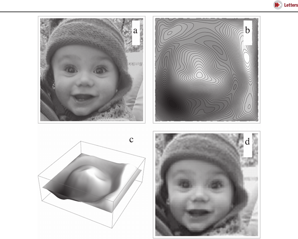
The method of creation of the magic windows using

(2.5) wil l be illustrated with reference to ﬁgure 4.The

desired i mage (ﬁgure 4(a)) is a smooth function I(R),with

0 {X, Y} 1, obtained by interpolating the 200× 200

pixels of a digi t a l photogr aph . I(R) is normali zed so t hat



∬

()

{}

XYIXYd d , 1.

xy0,1

If this is not done, solution

of (2.5) will generate a window proﬁle h(r) in which the

desired re li ef is superimpo s ed o n an overall pa rab ol oida l

proﬁle. With the normalized I(R) − 1, the window in (2.5) is

generat ed by standard pa r t ia l d ifferential equation software

(IusedMathematica’sNDSolve),withDirichletboundary

conditions chosen as a convenient way of removing t he

ambiguity represented by (2.6).Figures4(b) and (c) show

the resulting magic window proﬁle; the inverse Laplacian is

asmoothingoperation,sotheproﬁ le is a blur red version of

the desired image.

To simulate the image cast by this window, we evaluate

the Laplacian

 ()Rh

numerically. This is not very sensitive

to the discretization of the derivatives, and gives the result

shown in ﬁgure 4(d), nicely reproducing the starting picture

ﬁgure 4(a ).

Figure 2. Rays from proﬁle (3.1) calculated for n=1.5, (a) exactly from (2.1) and (2.2), and (b) approximately from the approximation (2.4).

Figure 3. Intensities corresponding to the exact and approximate rays in ﬁgure 2, for the indicated values of z. Dashed black curves represent

the exact intensities (2.3); the full red curves in (a)–(c) represent the approximate intensities (2.5), and in (d)–(f) the approximation (3.2) with

the unexpanded denominator.

J. Opt. 19 (2017) 06LT01

4. Concluding remarks

The scheme reported here, for creating magic windows, is

based on the Laplacian image. This is an approximation to

existing effective full geometrical-optics ray-tracing and

freeform inversion protocols. But the Laplacian image, and

the corresponding inversion procedure based on Poisson’s

equation, are extraordinarily simple and deserve to be

better known. If the underlying approximation is valid, the

Laplacian image applies to any family of rays or trajectories;

in particular, it has been applied to the interpretation of

electron-mictroscope images [24, 25].

The Laplace operator is the basis of a sharpening trans-

form, commonly used for edge detection [26–28]. Poisson’s

equation generates the inverse transform, which explains why

the magic window proﬁle h(r) is a smoothed version of the

desired image I(R), as already noted.

In common with most freeform optics, the Laplacian

image is an effect within ray theory: diffraction is neglected.

In the analogous magic mirror theory, it was shown that

diffraction effects are unimportant for the gently-varying

surfaces involved (appendix A of [4]—see also [29]).

Acknowledgments

I thank Professor David Jesson and Dr Howard Snelling for

discussions and encouragement. My research is supported by

a Leverhulme Trust Emeritus Fellowship and Leverhulme

Grant RPG-2016-181.

References

[1] Ayrton W E and Perry J 1878-9 The magic mirror of Japan

Proc. R. Soc. 28 127–48

[2] Mak S-Y and Yip D-Y 2001 Secrets of the Chinese magic

mirror replica Phys. Educ. 36 102–7

[3] Saines G and Tomilin M G 1999 Magic mirrors of the orient

J. Opt. Technol. 55 758–65

[4] Berry M V 2006 Oriental magic mirrors and the Laplacian

image Eur. J. Phys. 27 109–18

[5] Chu A K-H 2006 Comments on ‘oriental magic mirrors and the

Laplacian image’ Eur. J. Phys. 27 L13–5

[6] Seregin D A, Seregin A G and Tomilin M G 2004 Method of

shaping the front proﬁle of metallic mirrors with a given

relief of its back surface J. Opt. Technol. 71 121–2

Figure 4. (a) Desired image I(R); (b) contour plot of magic window proﬁle h(r); (c) 3D plot of magic window proﬁle; (d) simulated image

Lap

(R), calculated from (2.5). Copyright Miranda Berry-Bowen 2017, reproduced with permission.

J. Opt. 19 (2017) 06LT01

[7] Riesz F 2000 Geometrical optical model of the image

formation in Makyoh (magic-mirror) topography J. Phys.

D: Appl. Phys. 33 3033–40

[8] Rolland J P and Thompson K P 2012 Freeform optics:

Evolution? No, revolution!, http://spie.org/newsroom/

4309-freeform-optics-evolution-no-revolution

[9] Ball P 2013 Engineering light: pull an image from nowhere

New Sci. 217 40–3

[10] Miñano J C, Benítez P and Santamaría A 2009 Free-form

optics for illumination Opt. Rev. 16 99–102

[11] Paul y M 2012 Choreographing light EPFL Lausanne

Newsletter, http: //actu.epﬂ.ch/news/choreographing-

light/

[12] Schwartzburg Y, Testuz R, Tagliasacchi A and Pauly R 2014

High-contrast computational caustic design ACM Trans.

Graph. 33 74

[13] Brand M 2015 Lumographic lenses, http://zintaglio.com/

lens.html

[14] Gissibi T, Thiele S, Herkommer A and Giessen H 2016 Sub-

micrometre accurate free-form optics by three-dimensional

printing on single-mode ﬁbres Nat. Commun. 7 11763

[15] Fang F Z, Zhang X D, Weckenmann A, Zhang C X and

Evans C 2013 Manufacturing and me asurement o f freeform

optics CIRP Ann.— Manuf . Technol. 62

823–46

[16] Oliker V 2003 Mathematical aspects of design of beam-shaping

surfaces in geometrical optics Trends in Nonlinear Analysis ed

MKirkilioniset al (Berlin: Springer) pp 193–224

[17] Oliker V, Rubinstein J and Wolansky G 2015 Supporting

quadric meth od in optical design of freeform lenses for

illumination cont rol of a collimate d l igh t Adv. Appl. Math.

62 160–83

[18] Oliker V 2017 Controlling light with freeform multifocal lens

designed with supporting quadric method (SQM) Opt. Exp 25

A58–A72

[19] Wu R, Zheng Z, Li H and Liu X 2011 Constructing optical

freeform surfaces using unit tangent vectors of feature data

points J. Opt. Soc. Am. A 28 1880–8

[20] Song W, Cheng D, Liu Y and Wang Y 2015 Free-form

illumination of a refractive surface using multiple-faceted

refractors Appl. Opt. 54 E1–7

[21] Ries H and Muschaweck J 2001 Tailored freeform optical

surfaces J. Opt. Soc. Am. A 19 590–5

[22] Liu J, Benitz P and Miñano J C 2014 Single freeform surface

imaging design with unconstrained object to image mapping

Opt. Express 22 30538

[23] Kiser T and Pauly M 2012 Caustic Art (EPFL Technical Report,

Lusanne), https://infoscience.epﬂ.ch/record/196165

[

24] Kennedy S M, Zheng C S, Tang W X, Paganin D M and

Jesson D E 2010 Laplacian image contrast in mirror electron

microscopy Proc. R. Soc. A 466 2857–74

[25] Lynch D F, Moodie A F and O’Keefe M A 1975 n-Beam lattice

images: V. The use of the charge-density approximation in the

interpretation of lattice images Acta. Cryst. A31 300–6

[26] Marr D and Hildreth E 1980 Theory of edge detection Proc. R.

Soc. B 207 187–217

[27] Chen J S and Medioni G 1989 Detection, localization and

estimation of edges IEEE Trans. Pattern Anal. Mach. Intell.

11 191–8

[28] Baraniak R G 1995 Laplacian Edge Detection, http://owlnet.

rice.edu/~elec539/Projects97/morphjrks/laplacian.html

[29] Ricketts M N, Winston R and Oliker V 2015 Proc. SPIE 9572

957200

J. Opt. 19 (2017) 06LT01