
Wheaton Public Library - Excel Pivot Tables 2021
1
Microsoft Excel 2021 - Pivot Tables
What is a Pivot Table?
A Pivot Table is an interactive way to quickly summarize large amounts of data. Some of the capabilities of a
Pivot Table include:
• Organizing large amounts of data in many user-friendly ways
• Summarizing data by categories and subcategories
• Expanding and collapsing levels of data to focus your results
• Moving rows to columns or columns to rows (or “pivoting”) to see different summaries of the source data
• Filtering, sorting, and grouping the most useful and interesting subset of data
• Presenting concise, attractive, and annotated online or printed reports
1
Setting Up a Pivot Table – Do’s and Don’ts
• DO organize your source data in columns with unique headings
• DON’T leave empty rows or columns (empty cells are ok)
• DO have consistent data – watch for abbreviations (N. instead of North) and typos
Creating a Pivot Table
• Go to Insert → Pivot Table. Double-check to make sure the correct range
of data is selected, then click OK.
• You can import data from an external source, such as a database or
separate spreadsheet file.
• The Pivot Table can be placed in the same Sheet as the data, or in a
separate Sheet
o New Worksheet – creates a new sheet where the Pivot Table will
be located.
o Existing Worksheet – choose the cell reference (e.g. F6) where the
Pivot Table should start.
BAD PIVOT TABLE LAYOUT
Year
2019
Branch
2018
Branch
Name
Allen
1234
North
Barbara
5678
East
James
9012
West
GOOD PIVOT TABLE LAYOUT
Name
Branch
Year
Sales
Allen
North
2019
1234
Barbara
East
2018
5678
James
West
2019
9012

Wheaton Public Library - Excel Pivot Tables 2021
2
Arranging Your Pivot Table
• In a Pivot Table, a field is a category of data, such as name, total sales,
branch, etc. It is identical to the Heading or first row of your source data.
• In the Pivot Table Field List, select Fields to add to the Table in one of four
areas, Filters, Column Labels, Row Labels, and Values.
o Use the checkbox to the left of the field name.
▪ Text based fields will be added to the Row area
▪ Number based fields will be added to the Values area
o To move a field to a different area, click and drag.
o You can also drag the Field to an area, or drag a second copy of a
field. This helps when you need the data displayed in two different
ways (e.g. a Value and a percent of a value)
• Keep in mind, moving the Fields to different areas can result in different
results.
Formatting – Add visual elements to your Pivot Table
• Go to PivotTable Tools Design →Pivot Table Styles, and hover over a preset Style to preview how your
Pivot Table changes.
• Use the Pivot Table Style Options check boxes to add or remove Row/Column Headers and Banding
• Renaming Pivot Table Components
o Excel generally provides names for the Pivot Table title, column headings, etc. This can be
changed by going to PivotTable Tools Analyze → Pivot Table→ Pivot Table Name
o Fields can be renamed as well. First click on the heading you need to rename, and then go to
Pivot Table Tools Analyze → Active Field.
Data arranged by Columns
Data arranged by Rows

Wheaton Public Library - Excel Pivot Tables 2021
3
Expanding/Collapsing and Grouping
• A Pivot Table with a lot of data to summarize may get overwhelming on the
screen. Use Expand or Collapse to limit the amount of data visible at one
time.
o Next to each Row Label is a plus or minus sign. Click the plus sign to Or,
Go to PivotTable Tools Analyze→Active Field→Expand Field/Collapse
Field.
• Grouping – Allows you to select multiple items and then view them together (e.g. Science Fiction and
Fantasy could be grouped together, or you could divide the year into quarters by grouping months)
o Select the items.
o Go to PivotTable Tools Analyze → Group → Group Selection
Field Settings and Calculations
Summarizing Values – choose the way data is tabulated.
• Go to PivotTable Tools Analyze → Active Field → Field Settings → Summarize Values By Tab, or Right-
click the heading of any data field, then select Summarize Values By
o Sum – adds the data in a column or field (e.g. the total sales of the East Branch)
o Count – counts the number of items (e.g. the number of Nonfiction titles)
o Average, Max(imum), Min(imum), Product (multiplies)
Show Values As – create running totals or percentages of your data
• Go to PivotTable Tools Analyze → Active Field → Field Settings → Show Values As Tab, or Right-click the
heading of any data field, then select Show Values As.
No Calculation
Displays the value that is entered in the field.
% of Grand Total
Displays values as a percentage of the grand total of all the values or data points in the report.
% of Column Total
Displays all the values in each column or series as a percentage of the total for the column
or series
% of Row Total
Displays the value in each row or category as a percentage of the total for the row or
category.
% Of
Displays values as a percentage of the value of the Base item in the Base field.
% of Parent Row Total
Calculates values as follows: (value for the item) / (value for the parent item on rows)
% of Parent Column Total
Calculates values as follows: (value for the item) / (value for the parent item on columns)
% of Parent Total
Calculates values as follows:
(value for the item) / (value for the parent item of the selected Base field)
Difference From
Displays values as the difference from the value of the Base item in the Base field.
% Difference From
Displays values as the percentage difference from the value of the Base item in the Base
field.
Running Total in
Displays the value for successive items in the Base field as a running total.
% Running Total in
Calculates the value as a percentage for successive items in the Base field that are
displayed as a running total.
Wheaton Public Library - Excel Pivot Tables 2021
4
Rank Smallest to Largest
Displays the rank of selected values in a specific field, listing the smallest item in the field as 1,
and each larger value with a higher rank value.
Rank Largest to Smallest
Displays the rank of selected values in a specific field, listing the largest item in the field as 1,
and each smaller value with a higher rank value.
Index
Calculates values as follows: ((value in cell) x (Grand Total of Grand Totals)) / ((Grand Row
Total) x (Grand Column Total))
2
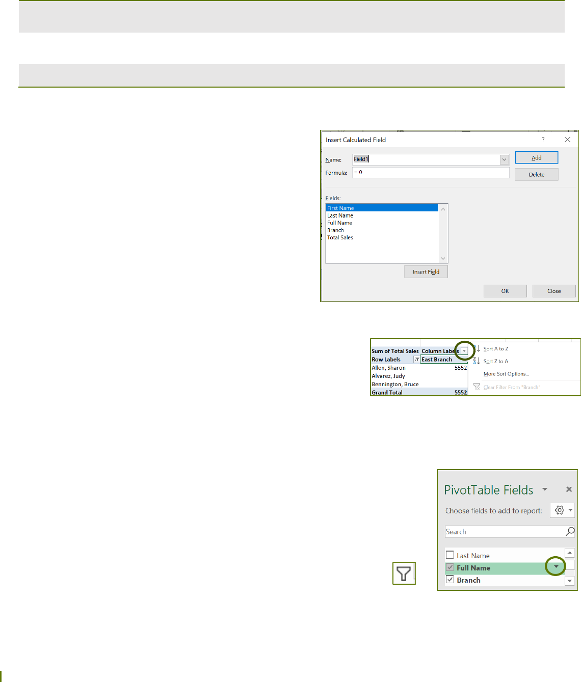
Fields, Items & Sets – create a formula in the Pivot Table
that did not exist in the original data.
• Go to Pivot Table Tools Analyze → Calculations →
Fields, Items & Sets → Calculated Field
• Assign a Name to the new field
• Formula – any recognized Excel formula is
acceptable, but you must type it in the formula field
(e.g. sum).
• Choose the Field or Fields that need to be
calculated, then click Insert Field.
Sorting and Filtering
Sorting - Alphabetically or numerically sort any column in the Pivot
Table.
• From the Row Headings/Labels cell, click the pull-down menu,
then select Sort A to Z/Sort Smallest to Largest or Sort Z to
A/Sort Largest to Smallest
• You can sort individual items in the column, or you can sort SubTotals.
Filtering – allows you to view or hide elements of the Pivot Table
Filter by Field List
• In the Field List, move your mouse to the far right and click on the arrow.
• Individual Items – check or uncheck individual items in a list. Check Select
All to toggle between all or none selected.
• Label Filters – used mostly to filter by text (e.g. all authors beginning with
“H”)
• Value Filters – used mostly to filter numbers (e.g. any values between 50 and
150)
• Fields that have a filter show a funnel on the right side of the Field List
• To remove the filter, click on the funnel, then click Clear Filter
Wheaton Public Library - Excel Pivot Tables 2021
5
Filter by Report – adds additional data fields to the Pivot Table in the form of a filter
• Drag fields to the Report Filter area
• The field appears at the top of the Pivot Table. Use the pull-down arrow to select individual items to filter.
• To remove the filter, click on the Report Filter at the top of the Pivot Table, and select
All.
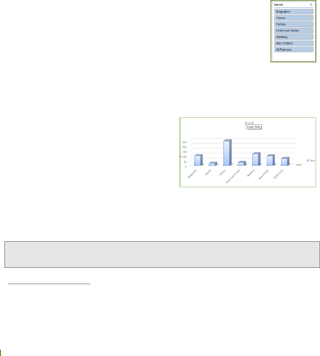
Slicer – displays the contents of a field for easier or multiple filtering
• Go to PivotTable Tools Analyze →Filter → Insert Slicer
• Select one or more categories. The slicer displays in a box near the Pivot Table.
• Go to Slicer Tools → Options for additional formatting and display options
Charts - Go to Pivot Table Tools Analyze → Tools → Pivot Chart
• Choose a Chart Style and then click OK
o NOTE: the following styles are NOT available from a Pivot Table: XY (Scatter), Stock, TreeMap,
Sunburst, Histogram, Box & Whisker, and Waterfall.
• Charts can be changed automatically by adding or removing fields, changing the order of data fields,
or creating filters.
Chart Options
• Analyze – make the Chart simpler or more
complicated by collapsing or expanding by fields.
Also allows you to insert slicers and perform
calculations
• Design – Change Chart type, switch row/column,
change Chart styles (color schemes)
• Format – change the background color, the size,
and the formatting of the Chart
IF YOU HAVE QUESTIONS, FEEL FREE TO EMAIL
1
Microsoft. (2020). Overview of PivotTable and PivotChart reports. Retrieved February 14, 2020, from Microsoft Office:
https://support.office.com/en-us/article/Overview-of-PivotTable-and-PivotChart-reports-527c8fa3-02c0-445a-a2db-7794676bce96
2
Microsoft. (2020).Show different calculations in PivotTable value fields. Retrieved February 14, 2020, from Microsoft Office:
https://support.office.com/en-us/article/Show-different-calculations-in-PivotTable-value-fields-014d2777-baaf-480b-a32b-
98431f48bfec
