
Changes
in
the
global
value
of
ecosystem
services
Robert
Costanza
a,
*
,
Rudolf
de
Groot
b
,
Paul
Sutton
c,d
,
Sander
van
der
Ploeg
b
,
Sharolyn
J.
Anderson
d
,
Ida
Kubiszewski
a
,
Stephen
Farber
e
,
R.
Kerry
Turner
f
a
Crawford
School
of
Public
Policy,
Australian
National
University,
Canberra,
Australia
b
Environmental
Systems
Analysis
Group,
Wageningen
University,
Wageningen,
The
Netherlands
c
Department
of
Geography,
University
of
Denver,
United
States
d
Barbara
Hardy
Institute
and
School
of
the
Natural
and
Built
Environments,
University
of
South
Australia,
Australia
e
University
of
Pittsburgh,
United
States
f
University
of
East
Anglia,
Norwich,
UK
1.
Introduction
Ecosystems
provide
a
range
of
services
that
are
of
fundamental
importance
to
human
well-being,
health,
livelihoods,
and
survival
(Costanza
et
al.,
1997;
Millennium
Ecosystem
Assessment
(MEA),
2005;
TEEB
Foundations,
2010;
TEEB
Synthesis,
2010).
Interest
in
ecosystem
services
in
both
the
research
and
policy
communities
has
grown
rapidly
(Braat
and
de
Groot,
2012;
Costanza
and
Kubiszewski,
2012).
In
1997,
the
value
of
global
ecosystem
services
was
estimated
to
be
around
US$
33
trillion
per
year
(in
1995
$US),
a
figure
significantly
larger
than
global
gross
domestic
product
(GDP)
at
the
time.
This
admittedly
crude
underestimate
of
the
welfare
benefits
of
natural
capital,
and
a
few
other
early
studies
(Daily,
1997;
de
Groot,
1987;
Ehrlich
and
Ehrlich,
1981;
Ehrlich
and
Mooney,
1983;
Odum,
1971;
Westman,
1977)
stimulated
a
huge
surge
in
interest
in
this
topic.
In
2005,
the
concept
of
ecosystem
services
gained
broader
attention
when
the
United
Nations
published
its
Millennium
Ecosystem
Assessment
(MEA).
The
MEA
was
a
four-year,
1300-
scientist
study
for
policymakers.
Between
2007
and
2010,
a
second
international
initiative
was
undertaken
by
the
UN
Environment
Programme,
called
the
Economics
of
Ecosystems
and
Biodiversity
(TEEB)
(TEEB
Foundations,
2010).
The
TEEB
report
was
picked
up
extensively
by
the
mass
media,
bringing
ecosystem
services
to
a
broader
audience.
Ecosystem
services
have
now
also
entered
the
consciousness
of
mainstream
media
and
business.
The
World
Business
Council
for
Sustainable
Development
has
actively
supported
and
developed
the
concept
(WBCSD,
2011,
2012).
Hundreds
of
projects
and
groups
are
currently
working
toward
Global
Environmental
Change
26
(2014)
152–158
A
R
T
I
C
L
E
I
N
F
O
Article
history:
Received
12
October
2013
Received
in
revised
form
18
February
2014
Accepted
1
April
2014
Keywords:
Ecosystem
services
Global
value
Monetary
units
Natural
capital
A
B
S
T
R
A
C
T
In
1997,
the
global
value
of
ecosystem
services
was
estimated
to
average
$33
trillion/yr
in
1995
$US
($46
trillion/yr
in
2007
$US).
In
this
paper,
we
provide
an
updated
estimate
based
on
updated
unit
ecosystem
service
values
and
land
use
change
estimates
between
1997
and
2011.
We
also
address
some
of
the
critiques
of
the
1997
paper.
Using
the
same
methods
as
in
the
1997
paper
but
with
updated
data,
the
estimate
for
the
total
global
ecosystem
services
in
2011
is
$125
trillion/yr
(assuming
updated
unit
values
and
changes
to
biome
areas)
and
$145
trillion/yr
(assuming
only
unit
values
changed),
both
in
2007
$US.
From
this
we
estimated
the
loss
of
eco-services
from
1997
to
2011
due
to
land
use
change
at
$4.3–20.2
trillion/yr,
depending
on
which
unit
values
are
used.
Global
estimates
expressed
in
monetary
accounting
units,
such
as
this,
are
useful
to
highlight
the
magnitude
of
eco-services,
but
have
no
specific
decision-making
context.
However,
the
underlying
data
and
models
can
be
applied
at
multiple
scales
to
assess
changes
resulting
from
various
scenarios
and
policies.
We
emphasize
that
valuation
of
eco-
services
(in
whatever
units)
is
not
the
same
as
commodification
or
privatization.
Many
eco-services
are
best
considered
public
goods
or
common
pool
resources,
so
conventional
markets
are
often
not
the
best
institutional
frameworks
to
manage
them.
However,
these
services
must
be
(and
are
being)
valued,
and
we
need
new,
common
asset
institutions
to
better
take
these
values
into
account.
ß
2014
Elsevier
Ltd.
All
rights
reserved.
*
Corresponding
author.
Tel.:
+61
02
6125
6987.
E-mail
addresses:
(R.
Costanza),
(R.
de
Groot),
(P.
Sutton),
(S.
van
der
Ploeg),
(S.J.
Anderson),
(I.
Kubiszewski),
(S.
Farber),
(R.K.
Turner).
Contents
lists
available
at
ScienceDirect
Global
Environmental
Change
jo
ur
n
al
h
o
mep
ag
e:
www
.elsevier
.co
m
/loc
ate/g
lo
envc
h
a
http://dx.doi.org/10.1016/j.gloenvcha.2014.04.002
0959-3780/ß
2014
Elsevier
Ltd.
All
rights
reserved.

better
understanding,
modeling,
valuation,
and
management
of
ecosystem
services
and
natural
capital.
It
would
be
impossible
to
list
all
of
them
here,
but
emerging
regional,
national,
and
global
networks,
like
the
Ecosystem
Services
Partnership
(ESP),
are
doing
just
that
and
are
coordinating
their
efforts
(Braat
and
de
Groot,
2012;
de
Groot
et
al.,
2011).
Probably
the
most
important
contribution
of
the
widespread
recognition
of
ecosystem
services
is
that
it
reframes
the
relation-
ship
between
humans
and
the
rest
of
nature.
A
better
understand-
ing
of
the
role
of
ecosystem
services
emphasizes
our
natural
assets
as
critical
components
of
inclusive
wealth,
well-being,
and
sustainability.
Sustaining
and
enhancing
human
well-being
requires
a
balance
of
all
of
our
assets—individual
people,
society,
the
built
economy,
and
ecosystems.
This
reframing
of
the
way
we
look
at
‘‘nature’’
is
essential
to
solving
the
problem
of
how
to
build
a
sustainable
and
desirable
future
for
humanity.
Estimating
the
relative
magnitude
of
the
contributions
of
ecosystem
services
has
been
an
important
part
of
changing
this
framing.
There
has
been
an
on-going
debate
about
what
some
see
as
the
‘‘commodification’’
of
nature
that
this
approach
supposedly
implies
(Costanza,
2006;
McCauley,
2006)
and
what
others
see
as
the
flawed
methods
and
questionable
wisdom
of
aggregating
ecosystem
services
values
to
larger
scales
(Chaisson,
2002).
We
think
that
these
critiques
are
largely
misplaced
once
one
under-
stands
the
context
and
multiple
potential
uses
of
ecosystem
services
valuation,
as
we
explain
further
on.
In
this
paper
we
(1)
update
estimates
of
the
value
of
global
ecosystem
services
based
on
new
data
from
the
TEEB
study
(de
Groot
et
al.,
2012,
2010a,b);
(2)
compare
those
results
with
earlier
estimates
(Costanza
et
al.,
1997)
and
with
alternative
methods
(Boumans
et
al.,
2002);
(3)
estimate
the
global
changes
in
ecosystem
service
values
from
land
use
change
over
the
period
1997–2011;
and
(4)
review
some
of
the
objections
to
aggregate
ecosystem
services
value
estimates
and
provide
some
responses
(Howarth
and
Farber,
2002).
We
do
not
claim
that
these
estimates
are
the
only,
or
even
the
best
way,
to
understand
the
value
of
ecosystem
services.
Quite
the
contrary,
we
advocate
pluralism
based
on
a
broad
range
of
approaches
at
multiple
scales.
However,
within
this
range
of
approaches,
estimates
of
aggregate
accounting
value
for
ecosystem
services
in
monetary
units
have
a
critical
role
to
play
in
heightening
awareness
and
estimating
the
overall
level
of
importance
of
ecosystem
services
relative
to
and
in
combination
with
other
contributors
to
sustainable
human
well-being
(Luisetti
et
al.,
2013).
2.
What
is
valuation?
Valuation
is
about
assessing
trade-offs
toward
achieving
a
goal
(Farber
et
al.,
2002).
All
decisions
that
involve
trade-offs
involve
valuation,
either
implicitly
or
explicitly
(Costanza
et
al.,
2011).
When
assessing
trade-offs,
one
must
be
clear
about
the
goal.
Ecosystem
services
are
defined
as
the
benefits
people
derive
from
ecosystems
–
the
support
of
sustainable
human
well-being
that
ecosystems
provide
(Costanza
et
al.,
1997;
Millennium
Ecosystem
Assessment
(MEA),
2005).
The
value
of
ecosystem
services
is
therefore
the
relative
contribution
of
ecosystems
to
that
goal.
There
are
multiple
ways
to
assess
this
contribution,
some
of
which
are
based
on
individual’s
perceptions
of
the
benefits
they
derive.
But
the
support
of
sustainable
human
well-being
is
a
much
larger
goal
(Costanza,
2000)
and
individual’s
perceptions
are
limited
and
often
biased
(Kahneman,
2011).
Therefore,
we
also
need
to
include
methods
to
assess
benefits
to
individuals
that
are
not
well
perceived,
benefits
to
whole
communities,
and
benefits
to
sustainability
(Costanza,
2000).
This
is
an
on-going
challenge
in
ecosystem
services
valuation,
but
even
some
of
the
existing
valuation
methods
like
avoided
and
replacement
cost
estimates
are
not
dependent
on
individual
perceptions
of
value.
For
example,
estimating
the
storm
protection
value
of
coastal
wetlands
requires
information
on
historical
damage,
storm
tracks
and
probability,
wetland
area
and
location,
built
infrastructure
location,
population
distribution,
etc.
(Costanza
et
al.,
2008).
It
would
be
unrealistic
to
think
that
the
general
public
understands
this
complex
connection,
so
one
must
bring
in
much
additional
information
not
connected
with
perceptions
to
arrive
at
an
estimate
of
the
value.
Of
course,
there
is
ultimately
the
link
to
built
infrastructure,
which
people
perceive
as
a
benefit
and
value,
but
the
link
is
complex
and
not
dependent
on
the
general
public’s
understanding
of
or
perception
of
the
link.
It
is
also
important
to
note
that
ecosystems
cannot
provide
any
benefits
to
people
without
the
presence
of
people
(human
capital),
their
communities
(social
capital),
and
their
built
environment
(built
capital).
This
interaction
is
shown
in
Fig.
1.
Ecosystem
services
do
not
flow
directly
from
natural
capital
to
human
well-
being
–
it
is
only
through
interaction
with
the
other
three
forms
of
capital
that
natural
capital
can
provide
benefits.
This
is
also
the
conceptual
valuation
framework
for
the
recent
UK
National
Ecosystem
Assessment
(http://uknea.unep-wcmc.org)
and
the
Intergovernmental
Platform
on
Biodiversity
and
Ecosystem
Services
(IPBES
–
http://www.ipbes.net).
The
challenge
in
ecosys-
tem
services
valuation
is
to
assess
the
relative
contribution
of
the
natural
capital
stock
in
this
interaction
and
to
balance
our
assets
to
enhance
sustainable
human
well-being.
The
relative
contribution
of
ecosystem
services
can
be
expressed
in
multiple
units
–
in
essence
any
of
the
contributors
to
the
production
of
benefits
can
be
used
as
the
‘‘denominator’’
and
other
contributors
expressed
in
terms
of
it.
Since
built
capital
in
the
economy,
expressed
in
monetary
units,
is
one
of
the
required
contributors,
and
most
people
understand
values
expressed
in
monetary
units,
this
is
often
a
convenient
denominator
for
expressing
the
relative
contributions
of
the
other
forms
of
capital,
including
natural
capital.
But
other
units
are
certainly
possible
(i.e.
land,
energy,
time,
etc.)
–
the
choice
is
largely
about
which
units
communicate
best
to
different
audiences
in
a
given
decision-
making
context.
3.
Valuation
is
not
privatization
It
is
a
misconception
to
assume
that
valuing
ecosystem
services
in
monetary
units
is
the
same
as
privatizing
them
or
commodifying
Fig.
1.
Interaction
between
built,
social,
human
and
natural
capital
required
to
produce
human
well-being.
Built
and
human
capital
(the
economy)
are
embedded
in
society
which
is
embedded
in
the
rest
of
nature.
Ecosystem
services
are
the
relative
contribution
of
natural
capital
to
human
well-being,
they
do
not
flow
directly.
It
is
therefore
essential
to
adopt
a
broad,
transdisciplinary
perspective
in
order
to
address
ecosystem
services.
R.
Costanza
et
al.
/
Global
Environmental
Change
26
(2014)
152–158
153

them
for
trade
in
private
markets
(Costanza,
2006;
Costanza
et
al.,
2012;
McCauley,
2006;
Monbiot,
2012).
Most
ecosystem
services
are
public
goods
(non-rival
and
non-excludable)
or
common
pool
resources
(rival
but
non-excludable),
which
means
that
privatiza-
tion
and
conventional
markets
work
poorly,
if
at
all.
In
addition,
the
non-market
values
estimated
for
these
ecosystem
services
often
relate
more
to
use
or
non-use
values
rather
than
exchange
values
(Daly,
1998).
Nevertheless,
knowing
the
value
of
ecosystem
services
is
helpful
for
their
effective
management,
which
in
some
cases
can
include
economic
incentives,
such
as
those
used
in
successful
systems
of
payment
for
these
services
(Farley
and
Costanza,
2010).
In
addition,
it
is
important
to
note
that
valuation
is
unavoidable.
We
already
value
ecosystems
and
their
services
every
time
we
make
a
decision
involving
trade-offs
concerning
them.
The
problem
is
that
the
valuation
is
implicit
in
the
decision
and
hidden
from
view.
Improved
transparency
about
the
valuation
of
ecosystem
services
(while
recognizing
the
uncertainties
and
limitations)
can
only
help
to
make
better
decisions.
It
is
also
incorrect
to
suggest
(McCauley,
2006)
that
conserva-
tion
based
on
protecting
ecosystem
services
is
betting
against
human
ingenuity.
Recognizing
and
measuring
natural
capital
and
ecosystem
services
in
terms
of
stocks
and
flows
is
a
prime
example
of
enlightened
human
ingenuity.
The
study
of
ecosystem
services
has
merely
identified
the
limitations
and
costs
of
‘hard’
engineer-
ing
solutions
to
problems
that
in
many
cases
can
be
more
efficiently
solved
by
natural
systems.
Pointing
out
that
the
‘horizontal
levees’
of
coastal
marshes
are
more
cost-effective
protectors
against
hurricanes
than
constructed
vertical
levees
(Costanza
et
al.,
2008)
and
that
they
also
store
carbon
that
would
otherwise
be
emitted
into
the
atmosphere
(Luisetti
et
al.,
2011)
implies
that
restoring
or
recreating
them
for
this
and
other
benefits
is
only
using
our
intelligence
and
ingenuity,
not
betting
against
it.
The
ecosystem
services
concept
makes
it
abundantly
clear
that
the
choice
of
‘‘the
environment
versus
the
economy’’
is
a
false
choice.
If
nature
contributes
significantly
to
human
well-being,
then
it
is
a
major
contributor
to
the
real
economy
(Costanza
et
al.,
1997),
and
the
choice
becomes
how
to
manage
all
our
assets,
including
natural
and
human-made
capital,
more
effectively
and
sustainably
(Costanza
et
al.,
2000).
4.
Uses
of
valuation
of
ecosystem
services
The
valuation
of
ecosystem
services
can
have
many
potential
uses,
at
multiple
time
and
space
scales.
Confusion
can
arise,
however,
if
one
is
not
clear
about
the
distinctions
between
these
uses.
Table
1
lists
some
of
the
potential
uses
of
ecosystem
services
valuation,
ranging
from
simply
raising
awareness
to
detailed
analysis
of
various
policy
choices
and
scenarios.
For
example,
Costanza
et
al.
(1997)
was
clearly
an
awareness
raising
exercise
with
no
specific
policy
or
decision
in
mind.
As
its
citation
history
verifies,
it
was
very
successful
for
this
purpose.
It
also
pointed
out
that
ecosystem
service
values
could
be
useful
for
several
of
the
other
purposes
listed
in
Table
1,
and
it
stimulated
subsequent
research
and
application
in
these
areas.
There
have
been
thousands
of
subsequent
studies
addressing
the
full
range
of
uses
listed
in
Table
1.
5.
Aggregating
values
Ecosystem
services
are
often
assessed
and
valued
at
specific
sites
for
specific
services.
However
some
uses
require
aggregate
values
over
larger
spatial
and
temporal
scales
(Table
1).
Producing
such
aggregates
suffers
from
many
of
the
same
problems
as
producing
any
aggregate
estimate,
including
macroeconomic
aggregates
such
as
GDP.
Table
2
lists
a
range
of
possible
approaches
for
aggregating
ecosystem
service
values
(Kubiszewski
et
al.,
2013a).
Basic
benefit
transfer,
the
technique
used
in
Costanza
et
al.
(1997)
assumes
a
constant
unit
value
per
hectare
of
ecosystem
type
and
multiplies
that
value
by
the
area
of
each
type
to
arrive
at
aggregate
totals.
This
can
be
improved
somewhat
by
adjusting
values
using
expert
opinion
of
local
conditions
(Batker
et
al.,
2008).
Benefit
transfer
is
analogous
to
the
approach
taken
in
GDP
accounting,
which
aggregates
value
by
multiplying
price
times
quantity
for
each
sector
of
the
economy.
Our
aggregate
is
an
accounting
measure
of
the
quantity
of
ecosystem
services
(Howarth
and
Farber,
2002).
In
this
accounting
dimension
the
measure
is
based
on
virtual
non-market
prices
and
incomes,
not
real
prices
and
incomes.
We
return
to
this
point
later
when
we
examine
some
of
the
criticisms
of
the
original
1997
study.
While
simple
and
easy,
this
approach
obviously
glosses
over
many
of
the
complexities
involved.
This
degree
of
approximation
is
appropriate
for
some
uses
(Table
1)
but
ultimately
a
more
spatially
explicit
and
dynamic
approach
would
be
preferable
or
essential
for
some
other
uses.
These
approaches
are
beginning
to
be
imple-
mented
(Bateman
et
al.,
2013;
Boumans
et
al.,
2002;
Burkhard
et
al.,
2013;
Costanza
et
al.,
2008;
Costanza
and
Voinov,
2003;
Crossman
et
al.,
2012;
Goldstein
et
al.,
2012;
Nelson
et
al.,
2009)
and
this
represents
the
cutting
edge
of
research
in
this
field.
Regional
aggregates
are
useful
for
assessing
land
use
change
scenarios.
National
aggregates
are
useful
for
revising
national
income
accounts.
Global
aggregates
are
useful
for
raising
awareness
and
emphasizing
the
importance
of
ecosystem
services
relative
to
other
contributors
to
human
well-being.
In
this
paper,
we
provide
some
updated
global
estimates,
recognizing
that
this
is
only
one
among
many
potential
uses
for
ecosystem
services
valuation,
and
that
this
use
has
special
requirements,
limitations,
and
interpretations.
6.
Estimates
of
global
value
Costanza
et
al.
(1997)
estimated
the
value
of
17
ecosystem
services
for
16
biomes
and
an
aggregate
global
value
expressed
in
monetary
units.
This
estimate
was
based
on
a
simple
benefit
transfer
method
described
above.
Notwithstanding
the
limitations
and
restrictions
in
benefit
transfer
techniques
(Brouwer,
2000;
Defra,
2010;
Johnston
and
Table
1
Range
of
uses
for
ecosystem
service
valuation.
Use
of
valuation
Appropriate
values
Appropriate
spatial
scales
Precision
needed
Raising
awareness
and
interest
Total
values,
macro
aggregates
Regional
to
global
Low
National
income
and
well-being
accounts
Total
values
by
sector
and
macro
aggregates
National
Medium
Specific
policy
analyses
Changes
by
policy
Multiple
depending
on
policy
Medium
to
high
Urban
and
regional
land
use
planning
Changes
by
land
use
scenario
Regional
Low
to
medium
Payment
for
ecosystem
services
Changes
by
actions
due
payment
Multiple
depending
on
system
Medium
to
high
Full
cost
accounting
Total
values
by
business,
product,
or
activity
and
changes
by
business,
product,
or
activity
Regional
to
global,
given
the
scale
of
international
corporations
Medium
to
high
Common
asset
trusts
Totals
to
assess
capital
and
changes
to
assess
income
and
loss
Regional
to
global
Medium
R.
Costanza
et
al.
/
Global
Environmental
Change
26
(2014)
152–158
154

Rosenberger,
2010)
it
is
an
attractive
option
for
researchers
and
policy-makers
facing
time
and
budget
constraints.
Value
transfer
has
been
used
for
valuation
of
environmental
resources
in
many
instances.
Nelson
and
Kennedy
(2009)
provide
a
critical
overview
of
140
meta-analyses.
de
Groot
et
al.
(2012)
estimated
the
value
of
ecosystem
services
in
monetary
units
provided
by
10
main
biomes
(Open
oceans,
Coral
reefs,
Coastal
systems,
Coastal
wetlands,
Inland
wetlands,
Lakes,
Tropical
forests,
Temperate
forests,
Woodlands,
and
Grasslands)
based
on
local
case
studies
across
the
world.
These
studies
covered
a
large
number
of
ecosystems,
types
of
landscapes,
different
definitions
of
services,
different
areas,
different
levels
of
scale,
time
and
complexity
and
different
valuation
methods.
In
total,
approximately
320
publications
were
screened
and
more
than
1350
data-points
from
over
300
case
study
locations
were
stored
in
the
Ecosystem
Services
Value
Database
(ESVD)
(http://www.fsd.nl/
esp/80763/5/0/50).
A
selection
of
665
of
these
value
data
points
were
used
for
the
analysis.
Values
were
expressed
in
terms
of
2007
‘International’
$/ha/year,
i.e.
translated
into
US$
values
on
the
basis
of
Purchasing
Power
Parity
(PPP)
and
contains
site-,
study-,
and
context-specific
information
from
the
case
studies.
We
added
some
additional
estimates
for
this
paper,
notably
for
urban
and
cropland
systems
(see
Supporting
Material
for
details).
A
detailed
description
of
the
ESVD
is
given
in
van
der
Ploeg
et
al.
(2010).
de
Groot
et
al.
(2012)
provides
details
of
the
results.
Below,
we
provide
a
comparison
of
the
de
Groot
et
al.
(2012)
results
with
the
Costanza
et
al.
(1997)
results
in
order
to
estimate
the
changes
in
the
flow
of
ecosystem
services
over
this
time
period.
After
some
consolidation
of
the
typologies
used
in
the
two
studies
we
can
compare
the
de
Groot
et
al.
(2012)
estimates
per
service
and
per
biome
with
the
Costanza
et
al.
(1997)
estimates
in
Table
3,
and
in
more
detail
in
Supporting
Material,
Table
S1.
Table
S1
lists
the
mean
value
for
each
service
and
biome
for
both
1997
and
2011.
Table
4
is
a
summary
of
the
number
of
estimates,
mean,
standard
deviation,
median,
and
minimum
and
maximum
values
used
in
de
Groot
et
al.
(2012).
All
values
are
in
international
$/ha/yr
and
were
derived
from
the
ESV
database.
Note
that
there
is
a
wide
range
of
the
number
of
studies
for
each
biome,
ranging
from
14
for
open
ocean
to
168
for
inland
wetlands.
This
is
a
significantly
larger
number
of
studies
than
were
available
for
the
Costanza
et
al.
study
(less
than
100).
One
can
also
note
the
wide
variation
and
high
standard
deviation
for
several
of
the
biomes.
For
example,
values
for
coral
reefs
varied
from
a
low
of
36,794
$/ha/yr
to
a
high
of
2,129,122
$/ha/yr.
Given
a
sufficient
number
of
studies,
some
of
this
variation
can
be
explained
by
other
variables.
For
example,
De
Groot
et
al.
performed
a
meta-regression
analysis
for
inland
wetlands
using
16
independent
variables
in
a
model
with
an
adjusted
R
2
of
0.442.
Variables
that
were
significant
in
explaining
the
value
of
inland
wetlands
included
the
area
of
the
study
site,
the
type
of
inland
wetland,
GDP/capita,
and
population
of
the
country
in
which
the
wetland
occurred,
the
proximity
of
other
wetlands,
and
the
valuation
method
used
for
the
study.
If
this
number
of
studies
were
available
for
the
other
biomes
in
our
global
assessment,
we
could
use
this
type
of
meta-regression
to
produce
more
accurate
estimates.
However,
for
the
current
estimate,
we
must
continue
to
rely
on
global
averages.
Global
averages
per
ha
may
vary
between
the
two
time
periods
we
are
comparing
for
three
distinct
reasons:
(1)
new
(and
generally
more
numerous
and
complete)
estimates
of
the
unit
values
of
ecosystem
services
per
ha;
(2)
changes
in
the
average
functionality
of
ecosystem
per
ha;
and
(3)
changes
in
value
per
ha
due
to
changes
in
human,
social,
or
built
capital.
The
actual
estimates
conflate
these
causes
and
we
see
no
way
of
disentangling
them
at
this
point.
However,
since
global
population
only
increased
by
16%
between
1997
and
2011
(from
5.83
to
7
billion),
and,
if
anything,
ecosystems
are
becoming
more
stressed
and
less
functional,
we
can
attribute
most
of
the
increase
in
unit
values
to
more
comprehensive,
value
estimates
available
in
2011
than
in
1997.
Table
3
shows
that
values
per
ha
estimated
by
de
Groot
et
al.
(2012)
are
an
average
of
8
times
higher
than
the
equivalent
estimates
from
Costanza
et
al.
(1997)
(both
converted
into
$2007).
Only
inland
wetlands
and
estuaries
did
not
show
a
significant
increase
in
estimated
value
per
ha,
but
these
were
among
the
best
studied
biomes
in
1997.
Some
biomes
showed
significant
increases
in
value.
For
example,
tidal
marsh/mangroves
increased
from
abound
14,000
to
around
194,000
$/ha/yr.
This
is
largely
due
to
new
studies
of
the
storm
protection,
erosion
control,
and
waste
treatment
values
of
these
systems.
Coral
reefs
also
increased
tremendously
in
estimated
value
from
around
8000
to
around
352,000
$/ha/yr
due
to
additional
studies
of
storm
protection,
erosion
protection,
and
recreation.
Cropland
and
urban
system
also
increased
dramatically,
largely
because
there
were
almost
no
studies
of
these
systems
in
1997
and
there
have
subsequently
been
several
new
studies
(Wratten
et
al.,
2013).
Table
3
also
shows
the
aggregate
global
annual
value
of
services,
estimated
by
multiplying
the
land
area
of
each
biome
by
the
unit
values.
Column
A
uses
the
original
values
from
Costanza
et
al.
(1997)
converted
to
2007
dollars
(total
=
$45.9
trillion/yr).
If
we
assume
that
land
areas
did
not
change
between
the
two
time
periods,
the
new
estimate,
shown
in
column
B
is
$145
trillion/yr,
are
more
than
3
times
larger
than
the
original
estimate.
This
is
due
solely
to
updated
unit
values.
However,
land
use
has
changed
significantly
between
the
two
years,
changing
the
supply
(the
flow)
of
ecosystem
services.
If
we
use
the
new
land
use
estimates
shown
in
Table
3
(see
Supporting
Material
for
details)
and
the
1997
unit
values,
we
get
the
estimates
in
column
C
–
a
total
of
$41.6
trillion/
yr.
Column
E
is
the
change
in
value
due
to
land
use
change
using
the
1997
unit
values.
Marine
systems
show
a
slight
increase
in
value,
while
terrestrial
systems
show
a
large
decrease.
This
decrease
is
largely
due
to
decreases
in
the
area
of
high
value
per
ha
biomes
(tropical
forests,
wetlands,
and
coral
reefs
–
shown
in
red
in
Table
3)
and
increases
in
low
value
per
ha
biomes.
The
total
net
decrease
is
estimated
to
be
$4.3
trillion/yr.
It
is
almost
certain
that
the
functionality
of
ecosystems
per
ha
has
also
declined
in
many
cases
so
the
supply
effects
are
surely
greater
than
this.
Column
D
Table
2
Four
levels
of
ecosystem
service
value
aggregation
(Kubiszewski
et
al.,
2013a,b).
Aggregation
method
Assumptions/approach
Examples
1.
Basic
value
transfer
Assumes
values
constant
over
ecosystem
types
Costanza
et
al.
(1997),
Liu
et
al.
(2010a,b)
2.
Expert
modified
value
transfer
Adjusts
values
for
local
ecosystem
conditions
using
expert
opinion
surveys
Batker
et
al.
(2008)
3.
Statistical
value
transfer
Builds
statistical
model
of
spatial
and
other
dependencies
de
Groot
et
al.
(2012)
4.
Spatially
explicit
functional
modeling
Builds
spatially
explicit
statistical
or
dynamic
systems
models
incorporating
valuation
Boumans
et
al.
(2002),
Costanza
et
al.
(2008),
Nelson
et
al.
(2009)
R.
Costanza
et
al.
/
Global
Environmental
Change
26
(2014)
152–158
155

shows
the
combined
effects
of
both
changes
in
land
areas
and
updated
unit
values.
The
net
effect
yields
an
estimate
of
$124.8
trillion/yr
–
2.7
times
the
original
estimate.
For
comparison,
global
GDP
was
approximately
46.3
trillion/yr
in
1997
and
$75.2
trillion/yr
in
2011
(in
$2007).
The
difference
between
columns
D
and
B
is
the
estimated
loss
of
ecosystem
services
based
on
land
use
changes
and
using
the
2011
unit
value
estimates.
This
is
shown
in
column
F.
In
this
case
marine
systems
show
a
large
loss
($10.9
trillion/yr),
due
mainly
to
a
decrease
in
coral
reef
area
and
the
substantially
larger
unit
value
for
coral
reef
using
the
2011
unit
values.
Terrestrial
systems
also
show
a
large
loss,
dominated
by
tropical
forests
and
wetlands,
but
countered
by
small
increases
in
the
value
of
grasslands,
cropland,
and
urban
systems.
Overall,
the
total
net
decrease
is
estimated
to
be
$20.2
trillion
in
annual
services
since
1997.
Given
the
more
comprehensive
unit
values
employed
in
the
2011
estimates,
this
is
a
better
approximation
than
using
the
1997
unit
values,
but
certainly
still
a
conservative
estimate.
The
present
value
of
the
discounted
flow
of
ecosystem
services
consumed
would
represent
part
of
the
stock
of
inclusive
wealth
lost/gained
over
time
(UNU-
IHDP,
2012).
As
we
have
previously
noted,
basic
value
transfer
is
a
crude
first
approximation
at
best.
We
could
put
ranges
on
these
numbers
based
on
the
standard
deviations
shown
in
Table
4,
but
there
are
other
sources
of
error
and
caveats
as
well,
as
described
in
Costanza
et
al.
including
errors
in
estimating
land
use
changes.
However,
we
think
that
solving
these
problems
will
most
likely
lead
to
even
larger
estimates.
For
example,
one
problem
is
the
limited
number
of
valuation
studies
available
and
we
expected
that
as
more
studies
became
available
from
1997
to
2011
the
unit
value
estimates
would
increase,
and
they
did.
We
also
anticipate
that
more
sophisticated
techniques
for
estimating
value
will
lead
to
larger
estimates.
For
example,
more
sophisticated
integrated
dynamic
and
spatially
explicit
modeling
Table
3
Changes
in
area,
unit
values
and
aggregate
global
flow
values
from
1997
to
2011
(green
are
values
that
have
increased,
red
are
values
that
have
decreased).
A. Origina
l
B.
Change
unit values
only
C. Change
area
only
D. Change
both unit
values and
area
E.
Column C -
Column A
F.
Column D -
Column B
Ass
uming
1997
area
and 1997
un
it
value
s
Ass
uming
1997
area
and 2011
un
it
value
s
Ass
uming
2011
area
and 1997
un
it
value
s
Ass
uming
2011
area
and 2011
un
it
value
s
Biome
egnahCegnahC
1997 2011
2011
-199
7
1997 2011
2011-1997
1997 201
1201
1 2011
1997
un
it
value
s 2011
un
it
value
s
Mari
ne 36,30
236,30
2 0
796
1,368 572 28
.9 60
.5 29
.5 49
.7 0.6 (10
.9)
Open Ocea
n33
,20
033
,200 0348 660
312 11
.6 21
.9 11
.6 21
.9 -
-
201,3201,3latsaoC
0
5,592
8,944
3,352 17.3 38
.6 18
.0 27
.7
0.6 (10
.9)
081seirautsE 180
031
,509 28,916 -2
,593
5.7
5.2
5.7
5.2
-
-
Seagrass/Algae
Bed
s200234 34 26,226 28,916
2,690
5.2
5.8
6.1
6.8
0.9
1.0
Coral
Ree
fs 62 28 -34
8,384 352,249 343
,865
0.5 21
.7
0.2
9.9 (0
.3) (11
.9)
066,2flehS
2,660 0
2,222
2,222
0
5.9
5.9
5.9
5.9
-
-
-
-
Terrestrial 15,32
3 15,32
3
0
1,109 4,901
3,792 17
.0 84
.5 12
.1 75
.1 (4
.9) (9
.4)
558,4tseroF 4,261 -594 1,338 3,800
2,462
6.5 19
.5
4.7 16
.2 (1.8) (3
.3)
009,1laciporT
1,258 -642
2,769
5,382
2,613
5.3 10
.2
3.5
6.8 (1
.8) (3
.5)
Tempera
te/Borea
l
2,955 3,003 48 417
3,137
2,720
1.2
9.3
1.3
9.4 0.0
0.2
Grass
/Rang
eland
s
3,898
4,418 520 321
4,166
3,845
1.2 16
.2
1.4 18
.4
0.2
2.2
033sdnalteW 188 -142 20,404 140,174 119
,770
6.7 36
.2
3.4 26
.4 (3.3) (9
.9)
Tidal
Mar
sh/Mangro
ves 165 128 -37 13
,786 193
,843 180
,057
2.3 32
.0
1.8 24
.8 (0
.5) (7
.2)
Swamps/Floodplain
s16560 -105 27,021 25,681 -1
,340
4.5
4.2
1.6
1.5 (2.8) (2
.7)
Lakes
/Rive
rs 20
0200011
,727 12
,512 785
2.3
2.5
2.3
2.5
-
-
529,1treseD
2,159 234
-
-
0
-
-
-
-
-
-
347ardnuT 433 -310
-
-
0
-
-
-
-
-
-
046,1046,1kcoR/ecI
0
-
-
0
-
-
-
-
-
-
004,1dnalporC
1,672 272 126
5,567
5,441
0.2
7.8
0.2
9.3
0.0
1.5
233nabrU 352 20
-
6,661
6,661
-
2.2
-
2.3
-
0.1
Total 51
,62
551
,62
5
0 45.9 145.0 41.6 124.8 (4.3)
(20.2)
(e6
ha)
2007$/ha/yr
Aggregate Global Flow Value
e12 2007$/yr
Unit valuesArea
e12
2007$
/yr
2011-1997
Change in Value
Table
4
Summary
of
the
number
of
estimates,
mean,
standard
deviation,
median,
minimum
and
maximum
values
used
in
de
Groot
et
al.
(2012).
Values
are
in
international
$/ha/yr,
derived
from
the
ESV
database.
No.
of
estimates
Total
of
service
means
(TEV)
Total
of
St.
Dev.
of
means
Total
of
median
values
Total
of
minimum
values
Total
of
maximum
values
Open
oceans
14
491
762
135
85
1664
Coral
reefs
94
352,915
668,639
197,900
36,794
2129,122
Coastal
systems
28
28,917
5045
26,760
26,167
42,063
Coastal
wetlands
139
193,845
384,192
12,163
300
887,828
Inland
wetlands
168
25,682
36,585
16,534
3018
104,924
Rivers
and
lakes
15
4267
2771
3938
1446
7757
Tropical
forest
96
5264
6526
2355
1581
20,851
Temperate
forest
58
3013
5437
1127
278
16,406
Woodlands
21
1588
317
1522
1373
2188
Grasslands
32
2871
3860
2698
124
5930
R.
Costanza
et
al.
/
Global
Environmental
Change
26
(2014)
152–158
156
techniques
have
been
developed
and
applied
at
regional
scales
(Barbier,
2007;
Bateman
et
al.,
2013;
Bateman
and
Jones,
2003;
Costanza
and
Voinov,
2003;
Goldstein
et
al.,
2012;
Nelson
et
al.,
2009).
However,
few
have
been
applied
at
the
global
scale.
One
example
is
the
Global
Unified
Metamodel
of
the
Biosphere
(GUMBO)
that
was
developed
specifically
to
simulate
the
integrated
earth
system
and
assess
the
dynamics
and
values
of
ecosystem
services
(Boumans
et
al.,
2002).
GUMBO
is
a
‘metamodel’
in
that
it
represents
a
synthesis
and
simplification
of
several
existing
dynamic
global
models
in
both
the
natural
and
social
sciences
at
an
intermediate
level
of
complexity.
It
includes
dynamic
feedbacks
among
human
technology,
economic
produc-
tion,
human
welfare,
and
ecosystem
goods
and
services
within
and
across
11
biomes.
The
dynamics
of
eleven
major
ecosystem
goods
and
services
for
each
of
the
biomes
have
been
simulated
and
evaluated.
A
range
of
future
scenarios
representing
different
assumptions
about
future
technological
change,
investment
strategies
and
other
factors,
have
been
simulated.
The
relative
value
of
ecosystem
services
in
terms
of
their
contribution
to
supporting
both
conventional
economic
production
and
human
well-being
more
broadly
defined
were
estimated
under
each
scenario.
The
value
of
global
ecosystem
services
was
estimated
to
be
about
4.5
times
the
value
of
Gross
World
Product
(GWP)
in
the
year
2000
using
this
approach.
For
a
current
global
GDP
of
$75
trillion/yr
this
would
be
about
$347
trillion/yr,
or
almost
three
times
the
column
D
estimate
in
Table
3.
This
is
to
be
expected
since
the
dynamic
simulation
can
include
a
more
comprehensive
picture
of
the
complex
interdependencies
involved.
It
is
also
important
to
note
that
this
type
of
model
is
the
only
way
to
potentially
assess
more
than
marginal
changes
in
ecosystem
services,
including
irreversible
thresholds
and
tipping
points
(Rockstro
¨
m
et
al.,
2009;
Turner
et
al.,
2003).
7.
Caveats
and
misconceptions
We
want
to
make
clear
that
expressing
the
value
of
ecosystem
services
in
monetary
units
does
not
mean
that
they
should
be
treated
as
private
commodities
that
can
be
traded
in
private
markets.
Many
ecosystem
services
are
public
goods
or
the
product
of
common
assets
that
cannot
(or
should
not)
be
privatized
(Wood,
2014).
Even
if
fish
and
other
provisioning
services
enter
the
market
as
private
goods,
the
ecosystems
that
produce
them
(i.e.
coastal
systems
and
oceans)
are
common
assets.
Their
value
in
monetary
units
is
an
estimate
of
their
benefits
to
society
expressed
in
units
that
communicate
with
a
broad
audience.
This
can
help
to
raise
awareness
of
the
importance
of
eco system
services
to
society
and
serve
as
a
powerful
and
essential
communication
tool
to
inform
better,
more
balanced
decisions
regarding
trade-offs
with
policies
that
enhance
GDP
but
damage
eco system
services.
Some
have
argued
that
estimating
the
global
value
of
ecosystem
services
is
meaningless,
because
if
we
lost
all
ecosystem
services
human
life
would
end,
so
their
value
must
be
infinite
(Chaisson,
2002).
While
this
is
certainly
true,
as
was
clearly
pointed
out
in
the
1997
paper
(Costanza
et
al.,
1997),
it
is
a
simple
misinterpretation
of
what
our
estimate
refers
to.
Our
estimate
is
more
analogous
to
estimating
the
total
value
of
agriculture
in
national
income
accounting.
Whatever
the
fraction
of
GDP
that
agriculture
contributes
now,
it
is
clear
that
if
all
agriculture
were
to
stop,
economies
would
collapse
to
near
zero.
What
the
estimates
are
referring
to,
in
both
cases,
is
the
relative
contribution,
expressed
in
monetary
units,
of
the
assets
or
activities
at
the
current
point
in
time.
Referring
to
Fig.
1,
human
well-being
comes
from
the
interaction
of
the
four
basic
types
of
capital
shown.
GDP
picks
up
only
a
fraction
of
this
total
contribution
(Costanza
et
al.,
2014;
Kubiszewski
et
al.,
2013b).
What
we
have
estimated
is
the
relative
contribution
of
natural
capital
now,
with
the
current
balance
of
asset
types.
Some
of
this
contribution
is
already
included
in
GDP,
embedded
in
the
contribution
of
natural
capital
to
marketed
goods
and
services.
But
much
of
it
is
not
captured
in
GDP
because
it
is
embedded
in
services
that
are
not
marketed
or
not
fully
captured
in
marketed
products
and
services.
Our
estimate
shows
that
these
services
(i.e.
storm
protection,
climate
regulation,
etc.)
are
much
larger
in
relative
magnitude
right
now
than
the
sum
of
marketed
goods
and
services
(GDP).
Some
have
argued
that
this
result
is
impossible,
wrongly
assuming
that
all
of
our
value
estimates
are
based
on
willingness-to-pay
and
that
that
cannot
exceed
aggregate
ability-to-pay
(i.e.
GDP).
But
for
it
to
be
impossible,
one
would
have
to
argue
that
all
human
benefits
are
marketed
and
captured
in
GDP.
This
is
obviously
not
the
case.
Another
example
is
the
many
other
types
of
goods
and
services
traded
on
‘‘black
markets’’
that
in
some
countries
far
exceed
GDP.
Moreover,
our
estimate
is
an
accounting
measure
based
on
virtual
not
real
prices
and
incomes
and
it
is
these
virtual
total
expenditures
that
should
not
be
exceeded
(Costanza
et
al.,
1998;
Howarth
and
Farber,
2002).
It
is
also
important
for
policy
to
evaluate
gains/losses
in
stocks
and
consequent
service
flows
(analogous
to
net
GDP).
The
discounted
present
value
of
such
stock/flow
changes
is
a
measure
of
a
component
of
inclusive
wealth
or
wellbeing.
8.
Conclusions
The
concepts
of
ecosystem
services
flows
and
natural
capital
stocks
are
increasingly
useful
ways
to
highlight,
measure,
and
value
the
degree
of
interdependence
between
humans
and
the
rest
of
nature.
This
approach
is
complementary
with
other
approaches
to
nature
conservation,
but
provides
conceptual
and
empirical
tools
that
the
others
lack
and
it
communicates
with
different
audiences
for
different
purposes.
Estimates
of
the
global
account-
ing
value
of
ecosystem
services
expressed
in
monetary
units,
like
those
in
this
paper,
are
mainly
useful
to
raise
awareness
about
the
magnitude
of
these
services
relative
to
other
services
provided
by
human-built
capital
at
the
current
point
in
time.
Our
estimates
show
that
global
land
use
changes
between
1997
and
2011
have
resulted
in
a
loss
of
ecosystem
services
of
between
$4.3
and
$20.2
trillion/yr,
and
we
believe
that
these
estimates
are
conser-
vative.
One
should
not
underestimate
the
importance
of
the
change
in
awareness
and
worldview
that
these
global
estimates
can
facilitate
–
it
is
a
necessary
precursor
to
practical
application
of
the
concept
using
changes
in
the
flows
of
services
for
decision-
making
at
multiple
scales.
It
allows
us
to
build
a
more
comprehensive
and
balanced
picture
of
the
assets
that
support
human
well-being
and
human’s
interdependence
with
the
well-
being
of
all
life
on
the
planet.
Acknowledgements
The
TEEB
study
was
funded
by
the
German,
UK,
Dutch,
Swedish,
Norwegian
and
Japanese
governments,
and
coordinated
by
UNEP
and
the
TEEB-offices
(UFZ,
Bonn,
Germany
and
in
Geneva,
Switzerland)
who
provided
financial
and
logistic
support
for
the
development
of
the
database.
We
thank
the
Crawford
School
of
Public
Policy
at
Australian
National
University
and
the
Barbara
Hardy
Institute
at
the
University
of
South
Australia
for
support
during
the
preparation
of
this
manuscript.
We
also
thank
four
anonymous
reviewers
for
their
helpful
comments
on
earlier
drafts.
Appendix
A.
Supplementary
data
Supplementary
data
associated
with
this
article
can
be
found,
in
the
online
version,
at
doi:10.1016/j.gloenvcha.2014.04.002.
R.
Costanza
et
al.
/
Global
Environmental
Change
26
(2014)
152–158
157
References
Barbier,
E.B.,
2007.
Valuing
ecosystem
services
as
productive
inputs.
Econ.
Policy
22,
177–229.
Bateman,
I.J.,
Harwood,
A.R.,
Mace,
G.M.,
Watson,
R.T.,
Abson,
D.J.,
Andrews,
B.,
Binner,
A.,
Crowe,
A.,
Day,
B.H.,
Dugdale,
S.,
Fezzi,
C.,
Foden,
J.,
Hadley,
D.,
Haines-Young,
R.,
Hulme,
M.,
Kontoleon,
A.,
Lovett,
A.A.,
Munday,
P.,
Pascual,
U.,
Paterson,
J.,
Perino,
G.,
Sen,
A.,
Siriwardena,
G.,
van
Soest,
D.,
Termansen,
M.,
2013.
Bringing
ecosystem
services
into
economic
decision-making:
land
use
in
the
United
Kingdom.
Science
341,
45–50.
Bateman,
I.J.,
Jones,
A.P.,
2003.
Contrasting
conventional
with
multi-level
modelling
approaches
to
meta-analysis:
expectation
consistency
in
UK
woodland
recrea-
tion
values.
Land
Econ.
79,
235–258.
Batker,
D.,
Swedeen,
P.,
Costanza,
R.,
de
la
Torre,
I.,
Boumans,
R.,
Bagstad,
K.,
2008.
A
New
View
of
the
Puget
Sound
Economy:
The
Economic
Value
of
Nature’s
Services
in
the
Puget
Sound
Basin.
Earth
Economics,
Tacoma,
WA.
Boumans,
R.,
Costanza,
R.,
Farley,
J.,
Wilson,
M.A.,
Portela,
R.,
Rotmans,
J.,
Villa,
F.,
Grasso,
M.,
2002.
Modeling
the
dynamics
of
the
integrated
earth
system
and
the
value
of
global
ecosystem
services
using
the
GUMBO
model.
Ecol.
Econ.
41,
529–560.
Braat,
L.,
de
Groot,
R.,
2012.
The
ecosystem
services
agenda:
bridging
the
worlds
of
natural
science
and
economics,
conservation
and
development,
and
public
and
private
policy.
Ecosyst.
Serv.
1,
4–15.
Brouwer,
R.,
2000.
Environmental
value
transfer:
state
of
the
art
and
future
prospects.
Ecol.
Econ.
32,
137–152.
Burkhard,
B.,
Crossman,
N.,
Nedkov,
S.,
Petz,
K.,
Alkemade,
R.,
2013.
Mapping
and
modelling
ecosystem
services
for
science,
policy
and
practice.
Ecosyst.
Serv.
4,
1–146.
Chaisson,
E.J.,
2002.
Cosmic
Evolution:
The
Rise
of
Complexity
in
Nature.
Harvard
University
Press,
Cambridge,
MA.
Costanza,
R.,
2000.
Social
goals
and
the
valuation
of
ecosystem
services.
Ecosystems
3,
4–10.
Costanza,
R.,
2006.
Nature:
ecosystems
without
commodifying
them.
Nature
443,
749.
Costanza,
R.,
d’Arge,
R.,
de
Groot,
R.,
Farber,
S.,
Grasso,
M.,
Hannon,
B.,
Limburg,
K.,
Naeem,
S.,
O’Neill,
R.V.,
Paruelo,
J.,
Raskin,
R.G.,
Sutton,
P.,
van
den
Belt,
M.,
1998.
The
value
of
ecosystem
services:
putting
the
issues
in
perspective.
Ecol.
Econ.
25,
67–72.
Costanza,
R.,
Daly,
M.,
Folke,
C.,
Hawken,
P.,
Holling,
C.S.,
McMichael,
A.J.,
Pimentel,
D.,
Rapport,
D.,
2000.
Managing
our
environmental
portfolio.
Bioscience
50,
149–155.
Costanza,
R.,
dArge,
R.,
de
Groot,
R.,
Farber,
S.,
Grasso,
M.,
Hannon,
B.,
Limburg,
K.,
Naeem,
S.,
Oneill,
R.V.,
Paruelo,
J.,
Raskin,
R.G.,
Sutton,
P.,
van
den
Belt,
M.,
1997.
The
value
of
the
world’s
ecosystem
services
and
natural
capital.
Nature
387,
253–260.
Costanza,
R.,
Kubiszewski,
I.,
2012.
The
authorship
structure
of
ecosystem
services
as
a
transdisciplinary
field
of
scholarship.
Ecosyst.
Serv.
1,
16–25.
Costanza,
R.,
Kubiszewski,
I.,
Ervin,
D.,
Bluffstone,
R.,
Boyd,
J.,
Brown,
D.,
Chang,
H.,
Dujon,
V.,
Granek,
E.,
Polasky,
S.,
Shandas,
V.,
Yeakley,
A.,
2011.
Valuing
ecological
systems
and
services.
F1000
Biol.
Rep.
3,
14.
Costanza,
R.,
Kubiszewski,
I.,
Giovannini,
E.,
Lovins,
H.,
McGlade,
J.,
Pickett,
K.E.,
Ragnarsdottir,
K.V.,
Roberts,
D.,
De
Vogli,
R.,
Wilkinson,
R.,
2014.
Time
to
leave
GDP
behind.
Nature
505,
283–285.
Costanza,
R.,
Pe
´
rez-Maqueo,
O.,
Martinez,
M.L.,
Sutton,
P.,
Anderson,
S.J.,
Mulder,
K.,
2008.
The
value
of
coastal
wetlands
for
hurricane
protection.
AMBIO:
J.
Hum.
Environ.
37,
241–248.
Costanza,
R.,
Quatrini,
S.,
Øystese,
S.,
2012.
Response
to
George
Monbiot:
The
Valuation
of
Nature
and
Ecosystem
Services
is
Not
Privatization.
Responding
to
Climate
Change
(RTCC).
Costanza,
R.,
Voinov,
A.,
2003.
Landscape
Simulation
Modeling:
A
Spatially
Explicit,
Dynamic
Approach.
Springer,
New
York.
Crossman,
N.,
Burkhard,
B.,
Nedkov,
S.,
2012.
Quantifying
and
mapping
ecosystem
services.
J.
Biodivers.
Sci.
Ecosyst.
Serv.
Manage.
8,
1–185.
Daily,
G.C.,
1997.
Nature’s
Services:
Societal
Dependence
on
Natural
Ecosystems.
Island
Press,
Washington,
DC.
Daly,
H.E.,
1998.
The
return
of
Lauderdale’s
paradox.
Ecol.
Econ.
25,
21–23.
de
Groot,
R.,
1987.
Environmental
functions
as
a
unifying
concept
for
ecology
and
economics.
Environmentalist
Summer
7,
105–109.
de
Groot,
R.,
Brander,
L.,
van
der
Ploeg,
S.,
Costanza,
R.,
Bernard,
F.,
Braat,
L.,
Christie,
M.,
Crossman,
N.,
Ghermandi,
A.,
Hein,
L.,
Hussain,
S.,
Kumar,
P.,
McVittie,
A.,
Portela,
R.,
Rodriguez,
L.C.,
ten
Brink,
P.,
van
Beukering,
P.,
2012.
Global
estimates
of
the
value
of
ecosystems
and
their
services
in
monetary
units.
Ecosyst.
Serv.
1,
50–61.
de
Groot,
R.,
Costanza,
R.,
Broeck,
D.V.D.,
Aronson,
J.,
Burkhard,
B.,
Gomez-Bag-
gethun,
E.,
Haines-Young,
R.,
Kubiszewski,
I.,
Muller,
F.,
Petrosillo,
I.,
Potschin,
M.,
Ploeg,
S.V.D.,
Zurlini,
G.,
2011.
A
global
partnership
for
ecosystem
services.
Solutions
2,
42–43.
de
Groot,
R.S.,
Fisher,
B.,
Christie,
M.,
Aronson,
J.,
Braat,
L.,
Haines-Young,
R.,
Gowdy,
J.,
Maltby,
E.,
Neuville,
A.,
Polasky,
S.,
Portela,
R.,
Ring,
I.,
2010.
Integrating
the
ecological
and
economic
dimensions
in
biodiversity
and
ecosystem
service
valuation.
In:
Kumar,
P.
(Ed.),
The
Economics
of
Ecosystems
and
Biodiversity:
Ecological
and
Economic
Foundations.
Earthscan,
London.
de
Groot,
R.S.,
Kumar,
P.,
van
der
Ploeg,
S.,
Sukhdev,
P.,
2010.
Estimates
of
monetary
values
of
ecosystem
services.
In:
Kumar,
P.
(Ed.),
The
Economics
of
Ecosystems
and
Biodiversity:
Ecological
and
Economic
Foundations.
Earthscan,
London.
Defra,
2010.
Improving
the
Use
of
Environmental
Valuation
in
Policy
Appraisal:
A
Value
Transfer
Strategy.
Defra,
London.
Ehrlich,
P.,
Ehrlich,
A.,
1981.
Extinction:
The
Causes
and
Consequences
of
the
Disappearance
of
Species.
Random
House,
New
York.
Ehrlich,
P.R.,
Mooney,
H.A.,
1983.
Extinction,
substitution,
and
ecosystem
services.
Bioscience
33,
248–254.
Farber,
S.C.,
Costanza,
R.,
Wilson,
M.A.,
2002.
Economic
and
ecological
concepts
for
valuing
ecosystem
services.
Ecol.
Econ.
41,
375–392.
Farley,
J.,
Costanza,
R.,
2010.
Payments
for
ecosystem
services:
from
local
to
global.
Ecol.
Econ.
69,
2060–2068.
Goldstein,
J.H.,
Caldarone,
G.,
Duarte,
T.K.,
Ennaanay,
D.,
Hannahs,
N.,
Mendoza,
G.,
Polasky,
S.,
Wolny,
S.,
Daily,
G.C.,
2012.
Integrating
ecosystem-service
tradeoffs
into
land-use
decisions.
Proc.
Natl.
Acad.
Sci.
U.S.A.
109,
7565–7570.
Howarth,
R.B.,
Farber,
S.,
2002.
Accounting
for
the
value
of
ecosystem
services.
Ecol.
Econ.
41,
421–429.
Johnston,
R.J.,
Rosenberger,
R.S.,
2010.
Methods,
trends
and
controversies
in
con-
temporary
benefit
transfer.
J.
Econ.
Surv.
24,
479–510.
Kahneman,
D.,
2011.
Thinking
Fast
and
Slow.
Farrar,
Straus
and
Giroux,
New
York.
Kubiszewski,
I.,
Costanza,
R.,
Dorji,
P.,
Thoennes,
P.,
Tshering,
K.,
2013.
An
initial
estimate
of
the
value
of
ecosystem
services
in
Bhutan.
Ecosyst.
Serv.
3,
e11–e21.
Kubiszewski,
I.,
Costanza,
R.,
Franco,
C.,
Lawn,
P.,
Talberth,
J.,
Jackson,
T.,
Aylmer,
C.,
2013.
Beyond
GDP:
measuring
and
achieving
global
genuine
progress.
Ecol.
Econ.
93,
57–68.
Liu,
S.,
Costanza,
R.,
Farber,
S.,
Troy,
A.,
2010a.
Valuing
ecosystem
services:
theory,
practice
and
the
need
for
a
trans-disciplinary
synthesis
Ecological
Economics
Reviews.
Book
Series:
Annals
of
the
New
York
Academy
of
Sciences,
vol.
1185.
,
pp.
54–78.
Liu,
S.,
Costanza,
R.,
Troy,
A.,
D’Aagostino,
J.,
Mates,
W.,
2010b.
Valuing
New
Jersey’s
ecosystem
services
and
natural
capital:
a
spatially
explicit
benefit
transfer
approach.
Environ.
Manage.
45,
1271–1285.
Luisetti,
T.,
Bateman,
I.J.,
Turner,
R.K.,
2011.
Testing
the
fundamental
assumption
of
choice
experiments.
Land
Econ.
87,
284–296.
Luisetti,
T.,
Jackson,
E.L.,
Turner,
R.K.,
2013.
Valuing
the
European
coastal
blue
carbon
storage
benefit.
Mar.
Pollut.
Bull.
71,
101–106.
McCauley,
D.J.,
2006.
Selling
out
on
nature.
Nature
443,
27–28.
Millennium
Ecosystem
Assessment
(MEA),
2005.
Ecosystems
and
Human
Well-
Being:
Synthesis.
Island
Press,
Washington,
DC.
Monbiot,
G.,
2012.
Putting
a
price
on
the
rivers
and
rain
diminishes
us
all.
The
Guardian.
Nelson,
E.,
Mendoza,
G.,
Regetz,
J.,
Polasky,
S.,
Tallis,
H.,
Cameron,
D.R.,
Chan,
K.M.A.,
Dailey,
G.C.,
Goldstein,
J.,
Dareiva,
P.M.,
Lansdorf,
E.,
Naidoo,
R.,
Ricketts,
T.H.,
Shaw,
M.R.,
2009.
Modeling
multiple
ecosystem
services,
biodiversity
conser-
vation,
commodity
production,
and
tradeoffs
at
landscape
scales.
Front.
Ecol.
Environ.
7,
4–11.
Nelson,
J.P.,
Kennedy,
P.E.,
2009.
The
use
(and
abuse)
of
meta-analysis
in
environ-
mental
and
natural
resource
economics:
an
assessment.
Environ.
Resour.
Econ.
42,
345–377.
Odum,
H.T.,
1971.
Environment,
Power
and
Society.
John
Wiley,
New
York.
Rockstro
¨
m,
J.,
Steffen,
W.,
Noone,
K.,
Persson,
A
˚
.,
Chapin,
F.S.,
Lambin,
E.F.,
Lenton,
T.M.,
Scheffer,
M.,
Folke,
C.,
Schellnhuber,
H.J.,
Nykvist,
B.,
de
Wit,
C.A.,
Hughes,
T.,
van
der
Leeuw,
S.,
Rodhe,
H.,
So
¨
rlin,
S.,
Snyder,
P.K.,
Costanza,
R.,
Svedin,
U.,
Falkenmark,
M.,
Karlberg,
L.,
Corell,
R.W.,
Fabry,
V.J.,
Hansen,
J.,
Walker,
B.,
Liverman,
D.,
Richardson,
K.,
Crutzen,
P.,
Foley,
J.A.,
2009.
A
safe
operating
space
for
humanity.
Nature
461,
472–475.
TEEB
Foundations,
2010.
The
Economics
of
Ecosystems
and
Biodiversity:
Ecological
and
Economic
Foundations.
Earthscan,
London
and
Washington.
TEEB
Synthesis,
2010.
Mainstreaming
the
Economics
of
Nature:
A
Synthesis
of
the
Approach,
Conclusions
and
Recommendations
of
TEEB.
Earthscan,
London
and
Washington.
Turner,
R.K.,
Paavola,
J.,
Cooper,
P.,
Farber,
S.,
Jessamy,
V.,
Georgiou,
S.,
2003.
Valuing
nature:
lessons
learned
and
future
research
directions.
Ecol.
Econ.
46,
493–510.
UNU-IHDP,
2012.
Inclusive
Wealth
Report:
Measuring
Progress
Toward
Sustain-
ability.
UNU-IHDP,
Bonn.
van
der
Ploeg,
S.,
De
Groot,
R.S.,
Wang,
Y.,
2010.
In:
Development,
F.F.S.
(Ed.),
The
TEEB
Valuation
Database:
Overview
of
Structure,
Data,
and
Results.
Wagenin-
gen,
The
Netherlands.
WBCSD,
2011.
Guide
to
Corporate
Ecosystem
Valuation:
A
Framework
for
Improv-
ing
Corporate
Decision-Making.
Geneva,
Switzerland.
WBCSD,
2012.
Biodiversity
and
Ecosystem
Services:
Scaling
Up
Business
Solutions.
Company
Case
Studies
that
Help
Achieve
Global
Biodiversity
Targets.
Geneva,
Switzerland.
Westman,
W.E.,
1977.
How
much
are
nature’s
services
worth?
Science
197,
960–964.
Wood,
M.C.,
2014.
Nature’s
Trust:
Environmental
Law
for
a
New
Ecological
Age.
Cambridge
University
Press,
Cambridge,
UK.
Wratten,
S.,
Sandhu,
H.,
Cullen,
R.,
Costanza,
R.,
2013.
Ecosystem
Services
in
Agricultural
and
Urban
Landscapes.
Wiley-Blackwell,
Oxford,
UK.
R.
Costanza
et
al.
/
Global
Environmental
Change
26
(2014)
152–158
158
Supporting Material
Details of Updated Unit Value Estimates
Table S1 shows the values for 17 ecosystem services in 16 ecosystems, both marine and
terrestrial. Ecosystems service values between 1997 and 2011 were compared; all values in
the table were converted to US$2007 (a 1.38 inflation conversion was used between 1997 and
2011). Rows with 1997 values for each of the ecosystem services come directly from the
Costanza et al 1997 paper. Rows with 2011 values come from three sources. Most values are
from de Groot et al. 2012 (no highlight). These were supplemented with a few values from
Costanza et al 1997 (yellow highlight) when no updates were available but the service had
obviously not disappeared and the 1997 estimate was still the best available. In addition we
added estimates for agricultural and urban systems that were not included in de Groot et al.
2012 directly from the ESV database (red highlight). Area weighted averages are shown for
some aggregated biomes. For example, the values for coastal are the area weighted averages
for estuaries, seagrass, coral reefs and shelf.
Because the ecosystem categories in de Groot et al. 2012 do not completely align with the
ones in this paper, some adjustments were made. These include making coastal wetlands
equivalent to tidal marshes/mangroves, inland wetlands equivalent to swamps/floodplains,
and not including woodlands as a separate category as they were incorporated into forests and
grasslands.
The four columns at the right show aggregate total values estimated by multiplying the area
figures by the unit values. In column A, the 1997 land cover areas were used and the 1997
unit values (in US$2007). The $US45.9 trillion is the $33 Trillion/yr result as in Costanza et
al. 1997 updated to $2007. In column B, the 1997 land cover areas were used but with the
2011 unit values, showing the difference the new values make when fourteen years of land
cover change is not considered. In column C, the 2011 land area was used multiplied by the
1997 unit values, showing the results if the values were not updated but the land cover
changed. In column D, both the 2011 land area and the 2011 unit values were used.
Areal extent of Global Land Cover
The approach to characterizing the type and areal extent of global land cover is
influenced by the need to attribute numerous and diverse economic valuation studies to
particular land cover types. The “new high-resolution data bases” described by Elaine
Matthews (1) is still very coarse by today’s standards (one degree by one degree or ~10,000
km
2
pixels at the equator). At this spatial resolution many land covers get lost by aggregation
(e.g. urban, riparian areas, and wetlands). Consequently we relied to a great extent on the
areal extent of land cover provided in other references for some land covers that are
important but can only be measured at finer spatial resolution (2-4) (Durr et al. 2011). For

this update we are taking a similar approach that is informed by the same basic principles.
We are obtaining best estimates of the same 16 basic land cover types: Open Ocean,
Estuaries, Seagrass/Algae Beds, Coral Reefs, Shelf, Tropical Forest, Temperate/Boreal
Forest, Grass/Rangelands, Tidal Marsh/Mangroves, Swamps/Floodplains, Lakes/Rivers,
Desert, Tundra, Ice/Rock, Cropland, and Urban.
The state of the art of global mapping of land cover has progressed significantly since
the mid 1990’s which has spawned a diverse assortment of land cover data products in a
diverse assortment of classification schemes and spatial resolutions. A brief perusal of the
USGS land cover institute’s web site provides a sense of these developments over the last 15
years (http://landcover.usgs.gov/landcoverdata.php). Our determination of the best global
representation of land cover relevant to this inquiry was the GlobCover data set produced by
the European Space Agency in partnership with the United Nations Food and Agriculture
Organization (http://www.esa.int/esaCP/SEMZ16L26DF_index_0.html). The GlobCover
classification scheme is a good match to the 1997 classification scheme and it includes
improved measures of the spatial extent of wetlands, water bodies, and urban areas. One
issue for utilizing the GlobCover measures of land cover was the lack of a category for
‘Tundra’. The GlobCover categories of ‘lakes/rivers’, ‘grassland/rangeland’ and ‘ice and
rock’ were all significantly higher than the areal extents used in the 1997 paper. We chose to
hold the areal extent of ‘ice/rock’ and ‘lakes/rivers’ constant and attribute the difference to
the ‘tundra’ category. This still represents a ‘loss’ of ‘tundra’ that is probably a classification
issue captured in the ‘grass/rangelands’ category.
This update of the areal extent of land cover would ideally only represent true
changes to the actual land surfaces of the earth that have taken place over the time span.
Nonetheless, some of the differences can undoubtedly be attributed simply to improvements
in our ability to map, classify, and measure the surface of the earth. The ‘urban’ category
provides a case in point. The land cover classification ‘urban’ can be discussed and argued
about at great length. In any case, the 1997 number of 337 million hectares represents an
estimate of terrestrial urbanization at roughly 2.2%. We know urban extent has increased
over the past 15 years despite the great discrepancies in measurements of urban extent (5).
Conservative MODIS based measures of urban extent are on the order of 65 million ha
(~0.5% of the land), the GlobCover dataset is 31 million ha (~0.24% of the land), and the
Global Rural-Urban Mapping Project (6)( estimates urban extent at 352 million hectares
(~2.74% of the land). We used the GRUMP number to show a modest (~4%) increase in
urban extent over the time period in question. The importance of the ‘urban’ category relative
to measures of the economic value of ‘natural’ capital manifests primarily in the idea that
human well-being is increased via the interaction of social, natural, built, and human capital
and ‘urban’ is the spatial location of a significant fraction of built, human, and social capital.
Conservative estimates of ‘urban’ consequently can dramatically minimize the nature of the
spatial interactions that occur between natural, human, social, and built capital.
Figure S1 shows global land cover converted to ecosystem service value using the 2011 unit
values shown in Table S1.
References
Worldwide Typology of Nearshore Coastal Systems: Defining the Estuarine Filter of River
Inputs to the Oceans Hans H. Dürr & Goulven G. Laruelle & Cheryl M. van Kempen &
Caroline P. Slomp & Michel Meybeck & Hans Middelkoop Estuaries and Coasts (2011)
34:441–458 DOI 10.1007/s12237-011-9381-y
!"# $"#%&''()*+,#-./0&.#1)2)'&'3/4#&45#.&4567+)8#4)*#(32(69)+/.7'3/4#5&'� &+) +#:/9#;.3< &')#
+'753)+"#="#>.3<"#?@@."#%)')/9/."#22,#ABA#C!DE F G"#
H"# I"#-"#J&3.)K,#$;/+K+')<#-)/29&@(K"##CL@9342)9,#M)*#N/9O,#HPPDG"#
F"# I"#5)#-9//',#Q74;'3/4+#/:#M&'79)8#$1&.7&'3/4#/:#M&'79)#34#$4139/4<)4'&.#R.&44342,#
%&4&2)<)4',#&45#S);3+3/4#%&O342"##CT/.')9+6M//95(/::,#-9/4342)4,#!DDHG"#
A"# UM$R6T>%>,#VW()#T/9.5#?'.&+#/:#>/9&.#I)):+X##CU43')5#M&'3/4+#$4139/4<)4'#R9/29&<<)#
T/9.5#>/4+)91&'3/4#%/43'/9342#>)4'9)#CUM$R6T>%>G,#HP!HG"#
Y"# ?"#L;(4)35)9,#%"#?"#Q93)5.,#S"#R/')9),#%&@@342#2./0&.#790&4#&9)&+#7+342#%ZS[L#YPP6<#5&'&8#
4)*#<)'(/5+#&45#5&'&+)'+#0&+)5#/4#\790&4#);/9)23/4+]"#I)</')#L)4+342#/:#$4139/4<)4'#
114,##CHP!PG "#
^"# >[$L[M"#C>)4')9#:/9#[4')94&'3/4&.#$&9'(#L;3)4;)#[4:/9<&'3/4#M)'*/9O#C>[$L[MG,#HPPAG,#1/."#
HP!H"#

CPI conv. 1997 to 2011 = 1.38
1997 2011
Area Area
Biome (e6 ha) (e6 ha)
1997 2011 1997 2011 1997 2011 1997 2011 1997 2011 1997 2011 1997 2011 1997 2011 1997 2011 1997 2011 1997 2011
Marine 36,302 36,302 48 - - 66 10 13 - - - - - 407 - - 583 294 0 0 - -
Open Ocean 33,200 33,200 53 65 163 163
Coastal 3,102 3,102 - - - 75 121 153 - - - - - 4,769 - - 5,074 1,693 2 1 - -
Estuaries 180 180 479 782 25,368 29,118
Seagrass/Algae Beds 200 234 479 25,368 26,223
Coral Reefs 62 28 1,188 3,795 16,991 153,214 80 85
Shelf 2,660 2,660 1,975 1,975
Terrestrial 15,323 15,323 6 4 62 277 136 62 100 122 152 136 52 95 5 62 158 26 205 1,476 11 15
Forest 4,855 4,261 - 4 194 711 3 19 3 3 4 143 132 100 14 14 498 66 120 120 - 9
Tropical 1,900 1,258 12 307 2,044 7 66 8 8 10 27 337 337 14 14 1,272 3 120 120 30
Temperate/Boreal 2,955 3,003 122 152 0 0 191 14 14 93 120 120
Grass/Rangelands 3,898 4,418 9 9 0 40 3 3 60 39 44 2 2 120 75 35 35
Wetlands 330 188 183 - - 200 6,264 4,596 21 1,789 5,244 959 - 3,507 - - - 577 5,765 111,345 - -
Tidal Marsh/Mangroves
165 128 65 2,538 5,351 1,217 3,929 45 9,240 162,125
Swamps/Floodplains 165 60 366 488 9,991 2,986 41 5,606 10,488 408 2,607 1,713 2,289 3,015
Lakes/Rivers 200 200 7,514 7,514 2,922 1,808 918 918
Desert 1,925 2,159
Tun dra 743 433
Ice/Rock 1,640 1,640
Cropland 1,400 1,672 411 400 107 532 397 19 22
Urban 332 352 905 16
Total 51,625 51,625 1851 55 944 6637 2455 1423 1539 1871 2335 2083 795 16249 73 955 23564 11056 3142 22625 162 227
Notes: Indicates values used in Costanza et al. 1997, converted to US$2007
1. Numbers in the body of the table are in $2007 ha-1 yr-1 Indicates values derived directly from the ESV database
Row and column totals are in e9 $ yr-1 Indicates values used in de Groot et al. 2012, coverted in US$2007
ie. Column totals (in e9 $/yr) are the sum of the products of the
per ha services in the table and the area of each biome,
not the sum of the per ha services themselves.
Table S1. Revised summary of average global value of annual ecosystem services.
Pollination
10
Treatment
Waste
9
1
Gas
Regulation
Regulation
Water
4
Regulation
Disturbance
3
Cycling
Nutrient
8
Regulation
Climate
2
Control
Erosion
6
Supply
Water
5
Formation
Soil
7

A. Original
B. Change unit
values only
C. Change
area only
D. Change both
unit values and
area
2007$/ha/yr 2007$/ha/yr
Ratios
1997 2011 1997 2011 1997 2011 1997 2011 1997 2011 1997 2011 1997 2011 1997 2011
2011/1997
1997 2011 2011 2011
11 10 1 15 30 120 1 25 - 32 10 369 103 17 796 1,368 1.72 28.9 60.5 29.5 49.7
7 7 21 93 0 8 5 319 105 348 660 1.89 11.6 21.9 11.6 21.9
53 46 11 172 128 405 5 203 - 322 113 903 85 202 5,592 8,944.04 1.60 17.3 38.6 18.0 27.7
108 180 194 719 2,384 35 12 180 526 256 40 43 31,509 28,916 1 5.7 5.2 5.7 5.2
194 2,384 3 12 180 256 43 26,226 28,916 1 5.2 5.8 6.1 6.8
7 7 10 16,210 304 677 37 22,000 33,048 4,150 96,302 1 12,535 8,384 352,257 42 0.5 21.7 0.2 9.9
54 54 94 94 3 3 97 97 2,222 2,222 1 5.9 5.9 5.9 5.9
12 63 9 675 54 685 64 87 7 591 51 469 27 56 1,109 4,901 4.42 17.0 84.5 12.1 75.1
3 169 - 619 59 270 191 152 22 448 91 953 3 1 1,338 3,800 2.84 6.5 19.5 4.7 16.2
11 39 45 200 435 84 57 1,517 154 867 2 2 2,769 5,382 1.94 5.3 10.2 3.5 6.8
6 235 862 69 299 34 181 50 989 3 1 417 3,137 7.52 1.2 9.3 1.3 9.4
31 31 1,214 79 1,192 54 0 1,214 2 26 167 321 4,166 12.99 1.2 16.2 1.4 18.4
- 303 419 12,452 354 952 146 416 - 243 793 2,199 1,215 636 20,404 140,174 6.87 6.7 36.2 3.4 26.4
233 17,138 643 1,111 224 358 311 908 2,193 13,786 193,843 14.06 2.3 32.0 1.8 24.8
948 605 2,455 65 614 68 539 99 678 2,211 2,430 1,992 27,021 25,681 0.95 4.5 4.2 1.6 1.5
57 106 317 2,166 11,727 12,512 1.07 2.3 2.5 2.3 2.5
- - - - - -
- - - - - -
- - - - - -
33 33 75 2,323 219 1,042 82 126 5,567 44.04 0.2 7.8 0.2 9.3
5,740 - 6,661 - 2.2 - 2.3
576 1341 171 10876 1913 14843 995 2226 109 10225 1125 20573 4161 1489 45.9 145.0 41.6 124.8
Genetic
Recreation
Cultural
Total Value
per ha
Total Value
per ha
17
15
16
Food
Materials
Production
Raw
14
13
Resources
Assuming 2011
area and 2011
unit values
Assuming
2011 area and
1997 unit
values
12
Refugia
Habitat/
Control
Biological
11
Assuming 1997
area and 2011
unit values
Assuming
1997 area and
1997 unit
values
(e12 2007$/yr)
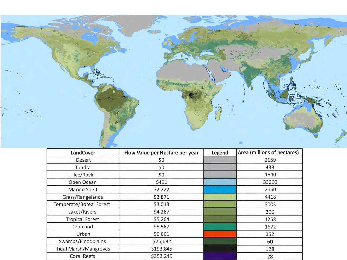
Figure S1. Map of global annual ecosystem services based on 2011 land areas and 2011 unit values!
